pip install numpy
pip install sympy
pip install PIL
pip install jupyter
pip install matplotlib1 Introduction to Python
Python was chosen to teach this course due to a number of advantages. In addition to being free, in the sense of open distribution and open-source code, it can be used on both Windows and Linux platforms. Furthermore, Python offers great versatility by providing numerous ready-to-use libraries while also allowing us to build new methods and functions. PyPI is the official Python repository where all libraries are stored. We can think of it as a GitHub for Python libraries. Python was created by Dutch programmer Guido van Rossum to be a simple, readable, and highly productive programming language. Python evolved and became a highly attractive language and a primary choice for web development, data analysis, and artificial intelligence applications, among others. Being genuinely an object-oriented language, it allows us to program with great efficiency and versatility, although it presents some differences in its implementation compared to other object-oriented languages. Another aspect that is very attractive in Python refers to the fact that it receives contributions from researchers all over the world in the form of libraries. This is a characteristic that drives a great development of the language in relatively short periods of time and enables us to find solutions for almost all problems we encounter in real situations. For the problems for which we cannot find solutions, the Python programming environment allows us to create our own solutions.
In these lecture notes, we intend to present the basic concepts of computational statistics in a very simple way. Initially, we will obtain our own solutions for a given method or technique, and in a second moment, we will show that we can have the same ready-made solution from Python when it is available. Particularly in this chapter, we will present some characteristics of the environment and the language to implement our solutions. Our course does not intend to provide advanced and maximally efficient solutions for the problems we will address, but rather to provide students with a first contact with the Python language and with the basic problems of computational statistics.
Some initial efforts are necessary before we can obtain any benefit. We do not intend to present in this course the Python resources for analyzing full or non-full rank linear models, non-linear models, generalized linear models, or graphs. Eventually, we may use some of these functions as an intermediate step to solve the problem for which we are presenting solutions. This material will be built with a brief and simplified theoretical approach to the topic and will associate practical examples of Python programming resources to solve a formulated problem, in particular cases of the studied theory.
This material is only a first version that will likely have many flaws. Thus, the reader who finds them or has a better solution to the problem can contribute by sending an email to danielff@ufla.br.
Visit my homepage https://des.ufla.br/~danielff/.
1.1 Introduction to Python Statements and Objects
In Python, objects can be of different types or structures, such as numbers (int, float, and complex), boolean, string, list, tuple, set, dictionary, functions (objects that encapsulate code), dataframes, and many others. We will succinctly and gradually describe some of these basic objects and statements.
Python statements can be written in a text editor and typed into the program’s terminal, but it is better to use appropriate IDEs. To use Python, we initially install a distribution of the Program. We recommend the current version which can be downloaded from the website https://www.python.org/ using the link https://www.python.org/ftp/python/3.15.1/python-3.15.1-amd64.exe. To type the codes, we recommend downloading the free program Positron from the website https://posit.co/ using the link https://cdn.posit.co/positron/releases/win/x86_64/Positron-2026.10.1-2-UserSetup-x64.exe.
See a screenshot of Positron:
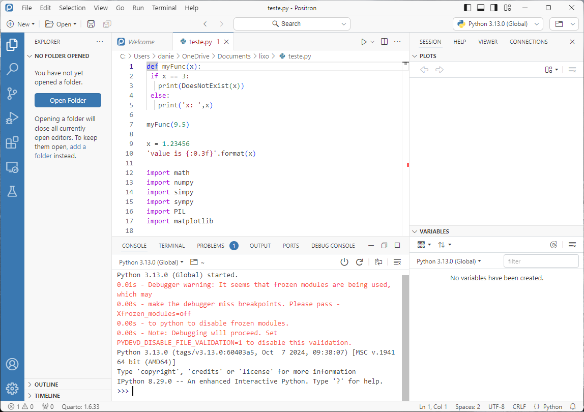
Python or ROnce installed, we can type the codes and with Ctrl Enter we execute the codes line by line or a block of highlighted lines. It is important to install some basic libraries if they are not already installed. Next, we have a code for this purpose.
Next, we must import the libraries we need. In the following script, we consider the importation of all previously installed libraries. The math library does not need to be installed, as it already comes with the Python distributions.
import math
import numpy
import sympy
import PIL
import jupyter
import matplotlib
WarningNote on the functionality of scripts in real-time
Important: The scripts of this new version will run in real-time in the html version. For some functionalities, some changes were necessary in the generated Python codes for html compatibility. Furthermore, some scripts require previous ones to be run in order to load specific objects or libraries so that they are functional and do not present error messages.
1.1.1 Basic Arithmetic Operations
We can use Python as a calculator. In the following script, each physical line of the editor has a specific statement, illustrating this usage mode. The statements presented are of the type: expression statements. We can separate several expression statements on the same line by separating them with a semicolon.
We can observe that the # symbol is used to insert comments in the code and the / operator performs division using real operators. For integer division, we can use //, so 6 // 5 returns \(1\) and 6 / 5 returns 1.2. The remainder of the integer division is obtained by the % operator. Thus, 6 % 5 returns 1. We also have that the ** operator is the power function, that is, for example, \(3^{10}\) is 3**10 in Python.
Python can also perform operations with complex numbers, which in this case, are represented by \(a+bj\), where \(a\) is the real part of the number and \(bj\) is the imaginary part, with \(j = \sqrt{-1}\). The \(j\) is represented by \(i\) in mathematics and other field books. The following program illustrates an operation with complex numbers given by \((6-4i)^2\). Thus, we have:
Below we present a script that makes use of the math library, whose first statement was to import it, the penultimate to obtain the value of \(\pi\), and the last one calculated \(\sqrt{2}\). We also performed another operation with complex numbers.
The NumPy and SymPy libraries are for various mathematical calculations, the latter performing symbolic calculations.
We can perform a basic mathematical operation like some of those presented above or even a more complex one and store the value in a variable, say x. These are assignment statements. The variable x can be used for other mathematical and even symbolic operations, if we use SymPy. See Knuth (1984) for a discussion on symbolic programming. The following script illustrates some cases of this procedure.
We assign data to Python variables. Python is case-sensitive, so names like X and x are different. In Python, variables are pointers. Assignments like \(x = 2\) create an object \(x\) and store the value \(2\) in it in other languages, but in Python, there is an integer object \(2\) and the variable \(x\) is a pointer pointing to it. See the consequences of this below, noting that \n performs a line break. There are no problems with scalar objects like these when we assign the same object to all of them and then change the assignment of one of them to another object (value). However, when it comes to, for example, lists, our next object to be studied, the issue is quite different.
To deal with complex number functions, the cmath library must be imported, and trigonometric functions of complex numbers can be used based on this library rather than math, which is designated for real numbers (float). See the illustrative script below.
1.2 Boolean Variables
Boolean variables point to True and False values only. Various comparison operations like ==, >=, <=, & (and), | (or), and ! (negation - not) can be used for this type of variable, the booleans. See a simple example of this. Later, we will return to talk about these boolean variable operators.
1.3 Strings
Strings (text variables) are an important type in Python. Once we have an object defined, the methods and functions are available to be used. Strings are denoted by str. See some examples, where strings were assigned or not to variables.
Some methods that we can use with strings are illustrated below, among many others, showing the power of the object-oriented language.
These methods act on the object, but as it was clear in the previous example, they do not change the content of the object. We can perform operations with strings, as illustrated below. The str.format method makes it possible to format strings, such as including substrings in the fields marked with {}.
If the user enters Daniel, the result will be Daniel was approved!. This version of Markdown does not yet support interactivity with the user. Therefore, the input was not evaluated in the output of this script. In the second statement, if the user enters a non-integer number, there will be an error message. There are options to deal with errors of this type and other causes as well.
To interact with the user, we use the input() function. It pauses the execution of the program and waits for a string to be typed on the keyboard.
See the standard code that would run in your local terminal (VS Code or Jupyter):
nome = input('enter your first name: ')
print(nome + ' was approved!')
x = int(input('enter an integer value: '))
  # transforms str into integer: int
x # if the input number is not int, it results in an error
WarningNote on
input()
Online environment: Since our book runs directly in your internet browser, the native input() function cannot open a keyboard dialog box synchronously.
In the interactive console below, we simulate the behavior of input() by defining the values directly in the variables input_nome and input_x. Change the texts in quotes to test the code behavior and the type conversion error:
1.4 Lists, Tuples, Sets and Dictionaries
We will cover each of these objects separately. Let’s start with lists.
1.4.1 Lists
Lists (lists) are the first building blocks for dealing with data manipulation. Lists are vectors whose first element starts at 0, but whose elements in each position can be of different types, from integers, booleans, reals, complex, strings, characters, sets, tuples, and other lists. Therefore, the list can be mixed, that is, contain different types of objects throughout its positions. Lists are part of the quartet list, tuple, set, and dictionary. The NumPy library provides additional tools for dealing with large collections of data.
The variable x is a list of integers with \(4\) elements, which are indexed by \(0\), \(1\), \(2\), \(3\). Thus, \(x[1]\) points to the value \(2\) and \(x[0]\) to the value \(1\). The variable y is also a list with \(4\) elements of different types, with \(y[0]\) being an integer, \(y[1]\) a string, \(y[2]\) a float, and \(y[3]\) a complex number. To create the list, we simply use the brackets [], with each element of the list separated by a comma. This statement is the list class constructor. It is possible to create a list with elements having repeated values, and they will be identified as being different, because the list respects and preserves the input order of the values. We can check if an element belongs to the list with in, as the following script shows, among other examples.
We can, in the same way as was done with strings, perform some arithmetic operations with lists, as shown in the example of the following script. These arithmetic operations do not act as mathematical arithmetic operations on Python lists. For example, y*2 duplicates the list y, creating a new list with the duplicated values. The operation x+y concatenates the two lists x and y, forming a new list.
Let’s now look at the problem of pointers, through the example of the script presented next.
We observe that if x, z, and b point to the same object, then if we change the value b[1] from 2 to 7, all three objects will be changed at position 1, which corresponds to the second value of the list, since it starts at position 0. However, if instead of b[1] = 7 we had used the assignment b = [7,9], then the vectors x and z would not be changed with the new assignment of vector b. In the previous examples, we also saw that the elements of a list are accessed by their index, which varies from 0 to n-1, where n is its length. Thus, the list x=[1,2,3,4] has its elements x[0] equal to 1, x[1] equal to 2, x[2] equal to 3, and x[3] equal to 4. We can also vary the index from -1 to -n, with -1 meaning the last position of the list, that is, position n-1, -2 corresponding to position n-2, and so on, until -n, which corresponds to position 0 of the list.
Lists are objects, and as such, we can use some methods associated with them. Lists are mutable and dynamic (we can change their elements), they are ordered (each element of the list has a defined order upon its creation), and they allow repeated elements. To use a method or a function, we must consider the difference between them. Although all methods are functions in Python, not every function is a method. Functions receive objects as inputs and do not modify them, while methods act on the objects. Below is a list of some methods or functions associated with lists:
sort(): sorts the list in ascending order.append(): adds an element to the end of the list.extend(): adds multiple elements to the list.index(): used to find the index of an element in the list.max(list): returns the maximum value of a list.min(list): returns the minimum value of a list.list(tuple): transforms atupleinto a list.len(list): returns the size of the list (number of elements).filter(fun,list): filters a list using a functionfun.
Let’s illustrate some of these methods with particular examples. We will consider a list and apply the sort() method to sort its values. In this example below, we will see the difference between a method and a function, observing how the method modifies the object that called it. In this case, a method call is given by the name of the list (object) followed by a dot and the name of the method: lista.met().
For the append method, we have the following script, which added the month of April to the end of a list with the first three months of the year.
The extend method is applied to the previous list x and adds two more elements to its end.
index() is a method to find the index of an element in the list. If the element sought is not in the list, Python will show an error message.
Functions len, max(), and min(), on the other hand, act on the argument of the function, but do not modify it. See the effect of these functions on the previously presented list x in the example.
To illustrate the use of filter(), let’s consider a function that returns True or False for a certain condition of interest. For example, if we wanted to know which numbers of the six elements of list x have a remainder of division by 2 less than 1.5. This result is obtained with the comparison a % 2 <= 1.5, which will return true or false for the number represented by a. But we must do this for all elements of the list x or any other list. We must create a function to receive each element of the list and check the condition, returning True or False. This is done by passing the list x or any other list through the filter() function to perform the intended iteration and comparison on its elements. Let’s create a first function and then apply the filter() function. The type of object returned from this function is filter, so the final result must be transformed into a list before printing.
We can use the constructor list(object) to construct a list from this object, as occurred with the object x_filtrado from the previous script. So list() is a list constructor. Note that the % operator returns the remainder of the integer division, which in this case, was by 2. The function resto returns true or false according to the condition of the remainder of the division of a by 2. To define a function we necessarily use def followed by the function name (resto) with the argument (a). Then comes the body of the function, which must have mandatory indentation. There is no separation with {} or [] or other characters to separate the body of the function. This separation is done solely using the appropriate indentations. We will talk more about functions in detail later.
We can take advantage of some ready-made list functions to calculate some quantities of interest, such as, for example, the sum of their elements. For this, we could use a loop structure, like the for loop that we will see later, and as the loop progresses, we update the sum. However, we can use the sum() function. A for loop is executed as interpreted bytecode, while the sum() function is written purely in the C language, therefore, much faster and more efficient. See the code below to illustrate the sum of all values of the vector x. We will talk about conditional and repetition structures later.
Other methods like count() (counts the number of occurrences of a given value), reverse() (sorts the list in reverse order to the original order), clear() (clears all data from the list), copy() (copies all data from the list), insert() (inserts an element at a specific position in the list), and pop() (removes an element at a specific position) are presented in the script below.
We can build a matrix using a list, since Python does not have a native matrix object. If we create a list of n components, with each of the components having m components, we will have an \(n \times m\) matrix. Let’s see in the script below the construction of the following matrix:
\[A = \left[ \begin{array}{cc} 1 & 4 \\ 2 & 5 \\ 3 & 6 \end{array} \right]. \tag{1.1}\]
The script corresponding to the matrix defined in (1.1) is:
We will also present some extra details to access the values of a list. We can access the value of a list x by indicating the position of the element we want to access as follows: x[i], where i represents an integer value between 0 and len(x)-1, say n-1, for lists of size n. To access a subset of a list L of size n, we can use the following statement L[m:s] which will access the elements from position m to position s-1 and not s. If the indices are negative, then the list will be accessed from back to front, with -1 corresponding to position n-1, -2 to position n-2, and so on, until -n, which corresponds to position 0. See some examples in the following script.
Accessing particular positions, for printing or for assignment:
Accessing positions with negative indices.
For blocks of elements we have that the statement L[m:s:r] accesses the elements at positions m, m+r, m+2r, ... until the (s-1)-th position or until the closest position to s-1 possible. Great care must be taken, because the upper limit does not indicate where the subset ends among the valid indices of a list, but rather, that it ends at the highlighted position subtracted by 1.
If we omit the lower or upper limits of the sequence, then the selected list will start at index 0 (initial value) or end at the last index (final value of the list), as in the last two examples presented.
1.4.2 Tuples
Tuples are objects very similar to lists. Several methods and functions that apply to lists also apply to tuples. Unlike lists, tuples are immutable objects, meaning that once created, they cannot be modified. If we create a tuple by t = (1,2,3) we cannot assign a value, for example, in this way: t[1] = 9. They can contain more than one identical value and are ordered, like lists. The way to create a tuple compared to a list is the use of parentheses instead of square brackets.
The count() and index methods can be used on tuples, as illustrated below. The index() method has the following syntax, with the last two arguments being optional: tuple.index(element, start, end).
The tuple can have any type as its elements, including a tuple or a list.
The question that arises is why should we use tuples if they cannot be modified? The answer to this comes from the fact that data manipulation via tuples, which are immutable, is much faster than with lists. Even though the tuple points to the same memory ID, we were able to modify one of its elements, which was the list in its second position. This did not change the memory ID that tuple t1 pointed to.
There are many methods or functions that work with tuples such as len(t) and count() as illustrated below.
The any(t) function returns True if there is any True item in the tuple and returns False otherwise. In this case, the tuple or any other appropriate type could have elements 0 and 1 or booleans. This function can be applied to lists, sets, and dictionaries.
We can also use the functions min(), max(), sum(), and sorted(), as illustrated below. The sorted() function sorts the tuple and returns a sorted list as a result. Note that the lista.sort() method alters the list object and cannot be applied to the tuple, because the tuple is immutable.
1.4.3 Sets
Set objects have a connotation very close to the definition in mathematics. These are sets in which the order or duplication of their elements do not change the set. They are immutable, unordered, and do not have identical elements in their occurrences. We can use the constructor set() to create a set or use curly braces {} to type its elements separated by a comma.
We cannot access an element of a set by B[0], for example, which causes an error, as can be seen in the result of the previous script. The order is not important, as can be verified by comparing the previous set A with the new set C created below.
Some mathematical operations with sets are available in Python, such as union, intersection, difference (\(A^c \cap B\)), and symmetric difference \(((A^c \cap B) \cup (A \cap B^c))\), as illustrated in the example below.
1.4.4 Dictionaries
Dictionaries (dictionary()) are mutable and iterable objects. Their elements always come in pairs, the first value being a key and the second element, the key’s value. Both the key and its value are Python objects. The key is immutable, but its associated values are mutable or immutable objects.
We have a dictionary, with keys 1, 2, and 3. For key 1 we have a list as its value, for key 2, we have a float value, and for key 3, we created a set object. Next, we add a key, named 4 with an associated boolean value. The keys() method retrieves the keys of the dictionary object D, transforms them into a list C, and prints the resulting list and its first element C[0].
Similarly, we can easily get the values of the keys, as illustrated in the script below. Later, we will see how we can use a for loop structure to iterate through the elements of the dictionary and store the values in a list or process them one by one.
We can delete the content of a key using the del function or using the pop() method. We can update the dictionary, creating new keys and values, with the update method.
We can create a dictionary object by creating two tuples, say c and v, with the keys and the key values (of the same size). Then we pair the elements with the zip(c, v) statement. Finally, we use the dict constructor to create the dictionary of paired values.
Thus, having access to a value from the list, we can use the appropriate methods and functions to deal with them. More details of these objects will appear in due course as we advance into the next chapters with more features of Python programming.
1.5 Matrices and Arrays
Matrices in Python, as we said and showed earlier, can be created by lists. Next, we will create a \(2 \times 2\) matrix using the list constructor to illustrate the creation procedure. If the dimension is just one, the lists are one-dimensional arrays, known as vectors.
To deal with vector (arrays) or matrix functions, we can, among other possibilities, use the NumPy library. Our first step is to import the NumPy library with the alias np, which is conventionally used to facilitate calling its methods and functions. This can only be done if we already have the NumPy library installed.
import numpy as npThen, we create a matrix using the array() and asarray() constructors. We will use our previous list A to do this to illustrate. It is important to note that lists accept data of various types, while NumPy lists or arrays are homogeneous structures more appropriate for mathematical and scientific calculations. Furthermore, calculations on NumPy arrays are vectorized, meaning we can perform element-by-element (vectorized) operations automatically and extremely fast. NumPy arrays are more efficient in memory usage because they store data in blocks and not as pointers where list data is scattered throughout memory.
We can also create the NumPy matrix from tuples, instead of lists. In addition, there are functions specific to the library to create matrices, such as, for example, the \(2 \times 4\) zero matrix below. There are also functions to create one-dimensional arrays (vectors), such as the arange(n, m) and linspace(n, m, s) methods. The first creates a vector going from n to the maximum m (integers) without including it by steps of \(1\), or from the minimum n to the maximum m (excluding the maximum) by steps of \(r\): arange(n,m) or arange(n,m,r). On the other hand, linspace(n,m,s) starts at n, ends at m, but with a step equal to (m - n) / (s - 1). Without specifying the s argument, as in this command linspace(n,m), NumPy uses the default value of 50 for it.
Let’s illustrate some simple calculations with vectors.
Matrix multiplication in turn can be done with the np.dot function, which has a method version as well, not modifying the object that triggered it.
Inverses can be obtained with the np.linalg.inv() function and the generalized Moore-Penrose inverses by the numpy.linalg.pinv() method. The determinant can be obtained by np.linalg.det() and the eigenvalues and eigenvectors (spectral decomposition) by np.linalg.eig(). It is important to note that the eigenvalues of np.linalg.eig() will not necessarily be sorted from largest to smallest, as is conventionally adopted in other programs. This method is very general and can be used on square real or complex matrices. Alternatively, for symmetric matrices NumPy has the np.linalg.eigh() method, which returns the eigenvalues in ascending order. See the example below.
We can also use the scipy library with the sp.linalg.eig() and sp.linalg.eigh() methods, which do exactly as their peers in the NumPy library. For this, we must import, after installing, the library using import scipy as sp.
For n x m matrices, we can use a matrix decomposition very useful for statistics, in methods such as principal components, AMMI, biplot, among others. This method is called singular value decomposition. In it we obtain the decomposition of a matrix \(\mathbf{A}\) (m x n) as follows: \(\mathbf{A}\) \(=\) \(\mathbf{U} \mathbf{\Lambda} \mathbf{V}^\top\), where the np.linalg.svd() method returns \(\mathbf{U}\) an \(m \times k\) orthonormal matrix by columns, \(\mathbf{V}\) an \(n \times k\) orthonormal matrix by columns and the vector corresponding to the diagonal of \(\mathbf{\Lambda}\), which is a \(k \times k\) diagonal matrix of real positive elements, if we use the full_matrices=False option. The matrices \(\mathbf{U}\) and \(\mathbf{V}\) are the singular vector matrices and the matrix \(\mathbf{\Lambda}\) is the singular value matrix, where \(k\) is the rank of \(\mathbf{A}\) which is \(k\le \min(n,m)\). The following script illustrates obtaining the singular decomposition of a \(3 \times 2\) matrix.
To verify that the decomposition is really adequate, we have the following script:
Many other functions exist in the NumPy library to deal with or operate on matrices. If we need some other function for some matrix operation, we will present it on those occasions.
1.6 Data Files
We will use this data structure little in this material, but we will make a brief introduction and explanation about the pandas library to deal with DataFrames. We will present the reading of a particular file with two variables X1 and X2, recorded as a text file separated by space between columns (variables). The path where this file is located on my computer is: g:/Meu Drive/daniel/Cursos/Estatistica computacional/Apostila/ and its name is dados.txt. We must initially install the pandas library with the statement: pip install pandas. Subsequently, we load the pandas library, as presented in the script below. To change the directory, we need to import the os library and use os.getcwd() to get the current working directory and to change it os.chdir('[path]').
import pandas as pd
import os

apath = os.getcwd() # project path
os.chdir('g:/Meu Drive/daniel/Cursos/Estatistica computacional/Apostila/')
print(os.getcwd())
g:\Meu Drive\daniel\Cursos\Estatistica computacional\ApostilaTo read a file from this directory into a DataFrame object, we can use the pd.read_csv('dados.txt',r'\s+') function, whose symbol r'\s+' means that the file is separated by spaces, and the number of spaces between columns from record (row) to record may vary, that is, if the number of spaces is not standardized between columns for the different lines of the data file.
# execute the previous script
dados = pd.read_csv('dados.txt',sep=r'\s+')
dados| X1 | X2 | |
|---|---|---|
| 0 | 13.4 | 14 |
| 1 | 14.6 | 15 |
| 2 | 13.5 | 19 |
| 3 | 15.0 | 23 |
| 4 | 14.6 | 17 |
| 5 | 14.0 | 20 |
| 6 | 16.4 | 21 |
| 7 | 14.8 | 16 |
| 8 | 15.2 | 27 |
| 9 | 15.5 | 34 |
| 10 | 15.2 | 26 |
| 11 | 16.9 | 28 |
| 12 | 14.8 | 24 |
| 13 | 16.2 | 26 |
| 14 | 14.7 | 23 |
| 15 | 14.7 | 9 |
| 16 | 16.5 | 18 |
| 17 | 15.4 | 28 |
| 18 | 15.1 | 17 |
| 19 | 14.2 | 14 |
DataFrames are tabular data structures, where each column consists of a sequence of values of the same type (boolean, float, strings, etc.), where the different columns can be and potentially are of different types. DataFrames have an additional column called index which in the previous example, of the dados object, varied from 0 to 19, because our DataFrame has 20 lines and two variables X1 and X2, which in the dados.txt file were identified in the first physical line of the file that was read by the read_csv() method. The index maps the lines of the DataFrame with the mentioned labels.
We will show how to build a DataFrame directly from a dict object for the pandas DataFrame() constructor. We will create a DataFrame of a completely randomized design, with 2 treatments and 3 replicates of each, with the respective yields evaluated in the 6 experimental plots.
We can add a new column to our DataFrame, or eliminate an existing one, creating a new DataFrame to receive the result, as shown below, with the columns option, for any order of the keys (column names).
To access the keys (columns), indices, and values of the DataFrame, we can use the following illustrative codes. We observe that the statement arqd.prod to access the prod column results in an error, because prod is a reserved word (product). We must use the previous alternative for this key.
To extract an entire row we use the loc method of the DataFrame associated with the row index (record), as illustrated in the following script.
To select a block of records (rows) going from inicio to fim (excluding the final limit) we use arqd[inicio:fim]. As illustrated below, where we extracted from index 0 to index 3, that is, the first three rows with indices 0, 1, and 2 of arqd.
Missing values can be part of the DataFrame, and in this case, they assume the value NaN, which stands for not a number. We can delete a column with the del statement, as follows.
We can filter by imposing specific conditions on the DataFrame. For example, if we were interested in the resulting DataFrame of elements where production is greater than or equal to 5, we would have the following result. The filtered result shows the records in the same original positions, and its original DataFrame arqd remains unchanged.
To save a DataFrame we can choose the directory (folder) and the file name and save it to a csv file (comma-separated file) with the statement arqd.to_csv('nome.csv,index=False, header=True) so as not to save the index and to save the header. We will recover in our code the original path with the statement os.chdir(apath), where apath was obtained when we started the topic about DataFrame and refers to the directory of this project. We chose the name dic.csv for the file. We can read the file again, as we showed in the first steps of the DataFrames approach. Once saved, we repeat its reading and place it in the dic object, where we must pay attention to the column separator, which in this case is the comma.
# execute the previous scripts
os.chdir(apath)
arqd.to_csv('dic.csv',index=False,header=True)
dic = pd.read_csv('dic.csv',sep=r',')
dic| rep | trat | prod | |
|---|---|---|---|
| 0 | 1 | 1 | 3.4 |
| 1 | 2 | 1 | 2.3 |
| 2 | 3 | 1 | 5.6 |
| 3 | 1 | 2 | 5.7 |
| 4 | 2 | 2 | 6.3 |
| 5 | 3 | 2 | 7.1 |
In future editions, we will show more details of DataFrames. In later chapters, if we come to need a DataFrame and some of its properties, then we will add the necessary contents at that time. We will now talk about conditional structures and repetition structures.
1.7 Programming Control Structures
Python is a programming environment in which programs contain modules, modules contain methods and functions, methods contain instructions, which create and process objects. These assignment statements are of the type a = b. We can call methods, functions, and use statements such as print(a), if/elif/else for action selection, for/else to perform iterations, while/else for loops in general, break and continue for loop control, def for defining functions and methods, yield for generator functions, among others. The statements are organized into expressions in groups of instructions, which unlike other languages are organized by indentation (paragraph indent). The body or group of instructions will be gathered together if they are indented in relation to the main instruction and with the same level of indentation. In other languages, instruction groups are gathered by curly braces: {groups of instructions}. The end of a line ends the statement, which can also be finalized by a semicolon. A statement can continue on a new line if the line ends with a \ or with the use of parentheses.
Variable names in Python must start with an underscore or letter, followed by numbers or letters or an underscore. Python differentiates uppercase from lowercase, so Y is different from y, for example. Names should avoid Python reserved words, such as False, None, True, class, and, if, elif, yield, while, break, global, nor, try, return, break, in, etc. By convention, classes in Python start with uppercase, and modules and variable names with lowercase.
Conditional structures, if/elif/else, are structures for selecting actions. This instruction can contain other instructions of the same type or different instructions in its groups. The general format is given by
if condition1:
  instructions1
elif condition2: # optional elif
  instructions2
else:            # optional else
    instructions3
The elif statement means else if and is optional. If condition1 is verified, the block named instructions1 (one or several lines of instructions) is executed, which are indented in relation to if. If the condition is false, condition2 is tested, and if it is true, the instructions denoted by instructions2 are executed, which can be a simple instruction or several instructions, indented in relation to elif. Finally, if condition2 is false, instructions3 are executed. Each line of the if, elif, or else statements is followed by a colon. See the simple example below.
For a probability model we have the following distribution function: \[\begin{align*} F_X(x) =& \left\{ \begin{array}{ll} 0 & \textrm{if } x < 0\\ x^2 & \textrm{if } 0\le x \le 1\\ 1 & \textrm{if } x > 1. \end{array} \right. \end{align*}\]
For this model, we have the following script, in which we decide which part of the program to run, according to the values assigned to x.
Repetition structures are for and while/else. There is also a third type of procedure in Python for performing iterations. The general structure of a code for the for loop is presented in the script below.
x = [1,2,3,4,5,6]
for i in x:
  instructions1
else:            # optional else instruction
  instructions2
The objects (x) of the for statement are the iterators or iterable objects, which are those that contain a countable number of values. Lists, tuples, dictionaries, and sets are all iterable objects. We will illustrate with a simple example below, to calculate the sum, product, and mean of a list of values.
To perform iterations on a dictionary, we have the following example:
Finally, an example on a set:
We can create a sequence of values with range(n) that goes from 0 to n-1. We can also use for on this sequence, as illustrated in the example below.
The while is another repetition structure, in which the block of indented instructions will be executed until a condition is met. The general structure is given below.
while condition:
  instructions1
else:            # optional else instruction
  instructions2
The example below illustrates calculating the total and average of a list.
We can use break and continue within the while (or the for). break is used after a second condition is met in the block of instructions inside the repetition structure and jumps the program’s execution to the first line of instruction after the loop block, that is, it ends the loop. continue executes the first line testing the primary condition of the while or taking the next iterator value in the for, that is, it goes to the beginning of the loop. See the example below.
We can use the filter function, as we have already illustrated earlier in this material, to perform iterations in our code. We will not give further details of this for now.
1.8 Functions
Functions in all languages are a powerful programming tool, which allows us to break down a large problem into small tasks (the functions), thus facilitating the resolution of the problem as a whole. We call this the divide-and-conquer strategy. Functions generally receive a variable (argument) and process it according to the rules defined in their instruction block. In this way, the language gains great power, convenience, and elegance. Learning to write useful functions is one of the many ways to make using Python comfortable and productive. The general syntax for a function is given by:
def name(arg1, arg2,...,argn):
  instructions
The instructions in the previous script mean a block of instructions (indented) and may or may not have the return object statement, which can occur in any part of the function or method’s instruction block. The function may not have a return, if it only modifies a file by saving a new result or if it prints a message when called. Arguments or parameters are passed to the function, and calling it must strictly follow the order in which they appear, unless the call is key-based, that is, of the type arg1 = 2.3, for example. In this case, the arguments can be placed in any order when calling the function. The arguments of a function can contain default values, that is, in the declaration of the function’s name we can have something like: def name(x, theta = 0.5). The argument theta=0.5 can be omitted when calling the function, and its default value of 0.5 will be assigned. By default, arguments with a default must obligatorily come last in the sequence of arguments.
We will present a simple function to test the hypothesis \(H_0: \mu=\mu_0\) from a simple sample of a normal distribution. Two arguments will be used: the data vector (list) \(x\) of size \(n\) and the hypothetical real value \(\mu_0\). The function will calculate the test statistic value \(t_c\) using: \[\begin{align}\label{ecp01:eq:tstudent} t_c = & \dfrac{\bar{X}-\mu_0}{\frac{S}{\sqrt{n}}}. \end{align}\]
The resulting function in Python is presented below. In this example, a sample of size \(n = 8\) was used to obtain the statistic’s value to test the hypothesis \(H_0: \mu=3.0\) (if the sample came from the Na’vi people). We can observe that the final result of the function is the statistic values and \(p\)-value, returned through a dictionary-type variable. This function uses in its scope three Python functions (basic NumPy functions) not yet presented. The first two, var() and mean(), return the variance and mean of the vector used as an argument, respectively, and the third, pt(), returns the cumulative probability of the Student’s \(t\) distribution for the first argument of the function with \(\nu\) degrees of freedom, which is its second argument.
We can rewrite this function to include a default value for the mu0 argument. If we chose the value 0 and in some function call this argument was omitted, the hypothesis test \(H_0: \mu=0\) would be performed by default.
Let’s perform a test for correlation in bivariate normal populations. Given a pair of vector variables X and Y taken on n individuals, we have the null hypothesis \[\begin{align*}
H_0:&\, \rho=0
\end{align*}\] and the test statistic under \(H_0\) given by \[\begin{align*}
t_c =& \dfrac{r\sqrt{n-2}}{\sqrt{1-r^2}},
\end{align*}\] where \(r\) is the sample correlation coefficient between \(X\) and \(Y\), and \(n\) is the sample size. Under \(H_0\), this statistic follows a Student’s \(t\) distribution with \(\nu=n-2\) degrees of freedom.
The function should receive the vectors \(\mathbf{x}\) and \(\mathbf{y}\) and return the result of the test: statistic and \(p\)-value. One can use the cor function from SciPy to obtain the correlation between \(\mathbf{x}\) and \(\mathbf{y}\).
Finally, let’s get a function to obtain real powers of positive definite symmetric square matrices. Consider a symmetric and positive definite matrix \(\mathbf{A}\): \[\begin{align*} \mathbf{A}=& \mathbf{P}\mathbf{\Lambda} \mathbf{P}^\top, \end{align*}\] then the power of order \(\alpha\in \mathbb{R}\) is given by \[\begin{align*} \mathbf{A}^\alpha=& \mathbf{P} \mathbf{\Lambda}^\alpha \mathbf{P}^\top. \end{align*}\]
It should receive \(\mathbf{A}\) and return \(\mathbf{A}^\alpha\). The following script illustrates a function to obtain these matrix powers. Note that it is not an element-by-element power. We must also note that it is not important that the eigenvalues are ordered. But it is obvious that the eigenvectors associated with each eigenvalue must be properly associated and preserved, and this is done by the NumPy library through the eig() function.
1.9 Computational Statistics
Computationally intensive methods have played an increasingly important role in solving problems in different areas of science. We will present algorithms to generate realizations of random variables from various univariate and multivariate probability distributions, to perform matrix operations, to perform inferences using permutation and bootstrap methods, etc. Thus, we seek to carry out a division of this material into a basic section and an applied section. Computational techniques are called computational statistics if they are used to perform inferences, to generate realizations of random variables, or to compare statistical methods and techniques.
We will explore methods of generating realizations of random variables of various probability models, to manipulate matrices, to obtain quadratures of distribution functions of various probability models and special functions in statistics, and finally, we will present computationally intensive methods to perform inferences in different real situations. We intend to create algorithms in the Python language and later, when they exist, present the instructions for accessing the same algorithms already implemented.
We will present the bootstrap and Monte Carlo methods, permutation tests, and the jackknife procedure to perform inferences in the most varied real situations. This course has basically two primary intentions. The first is to enable students to perform their own simulations and, the second, to allow them to perform their inferences of interest in situations where using classical inference would be highly complex.
Whether in frequentist inference or Bayesian inference, simulation methods for random numbers of different probability models assume great importance. To use computational statistics more efficiently, a minimum knowledge of simulating random variable realizations is a necessity that should not be ignored. We will place a great emphasis on this subject without neglecting the others. We will present in this material several algorithms developed and adapted for the Python language.
Simulating is the art of building models according to Naylor et al. (1971), with the objective of imitating the functioning of a real system, to verify what would happen if alterations were made to its operation (Dachs (1988)). This type of procedure can have a low cost, avoid losses by not using inadequate procedures, and optimize the decision and functioning of the real system.
Precautions against errors must be taken when we carry out some type of simulation. We can enumerate:
inadequate choice of distributions;
inadequate simplification of reality; and
implementation errors.
We must make the simulated system operate under the conditions of the real system and verify through some tests if the results are in agreement with what is observed in the real system. We call this process validation. Simulation is a technique we use to solve problems. If the achieved solution is faster, with equal or superior efficiency, of lower cost, and easy to interpret compared to any other method, the use of simulation is justifiable.
1.10 Exercises
Create in
Pythonthe vectors \(\mathbf{a}^\top=[4, 2, 1, 5]\) and \(\mathbf{b}^\top=[6, 3, 8, 9]\) and concatenate them forming a single vector. Obtain the vector \(\mathbf{c}=2\mathbf{a} - \mathbf{b}\) and the scalar \(d\) \(=\) \(\mathbf{b}^\top \mathbf{a}\). Create a sequence whose initial value is equal to \(2\) and the final value is \(30\) and whose step is equal to \(2\). Replicate each value of the sequence \(4\) times in two different ways (replicated values are aggregated, and the whole sequence replicates without equal values being aggregated).Select the subvector of \(\mathbf{x}^\top=[4, 3, 5, 7, 9, 10]\) whose elements are less than or equal to \(7\).
Create the matrix \[\begin{align*} \mathbf{A}= \left[\begin{array}{cc} 10 & 1 \\ 1 & 2 \end{array} \right] \end{align*}\] and determine the eigenvalues and the spectral decomposition of \(\mathbf{A}\).
Construct a function to verify how many elements of an \(n\)-dimensional vector are less than or equal to a real constant \(k\). Use the repetition structures
forandwhileto perform such a task (each of these structures must be implemented in a different function). Is there a more efficient procedure to generate such a function without using repetition structures? If yes, implement it.Implement a function to perform Student’s \(t\)-test for two independent samples. Consider the cases of heterogeneous and homogeneous variances. Use a conditional structure to apply the appropriate test, whether the variances are heterogeneous or homogeneous. The decision must be based on a test of homogeneity of variances. To perform this task, implement a specific function assuming normality of random samples.
Create a function to obtain the Moore-Penrose inverse of any \(n\) \(\times\) \(m\) matrix, based on the singular value decomposition, function
svdofnp.linalg.svd. For this, let there be a matrix \(\mathbf{A}\), whose singular value decomposition is \(\mathbf{A}\) \(=\) \(\mathbf{U}\mathbf{D}\mathbf{V}^\top\), in which \(\mathbf{D}\) is the diagonal matrix of the singular values and \(\mathbf{U}\) and \(\mathbf{V}\) are the corresponding singular vectors. The Moore-Penrose inverse of \(\mathbf{A}\) is defined by \(\mathbf{A}^+\) \(=\) \(\mathbf{V}\mathbf{D}^{-1}\mathbf{U}^\top\).