In this chapter, we present general methods for generating realizations of random variables from other probability distributions, such as exponential, normal, and binomial models. We will implement several functions in Python and conclude by presenting optimized, ready-to-use routines available in standard libraries.
3.1 Introduction
From this point forward, we will study one of the primary methods—governed by the fundamental law of probability transformation—for generating data from continuous or discrete probability distributions. For specific cases, we will illustrate alternative procedures that are efficient and computationally simpler. This transformation relies on the continuous uniform distribution \((0, 1)\) as its foundational model. For this reason, generating continuous uniform numbers is of paramount importance.
Later in these lecture notes, we will examine algorithms to numerically obtain the cumulative distribution function \(F(x)\) and its inverse function \(x = F^{-1}(p)\), where \(p\) belongs to the interval from \(0\) to \(1\). This knowledge is essential for applying this primary method.
In this chapter, we limit ourselves to presenting the theory for a few probability models for which we can easily obtain the cumulative distribution function and its inverse analytically. For more complex models, although the method based on the fundamental law of probability transformation is conceptually appropriate, we present only alternative methods, as it is generally inefficient in terms of the computation time required to generate each realization of the random variable. This inefficiency stems from having to compute the inverse cumulative distribution function numerically for complex probability models.
3.2 General Methods for Generating Realizations of Random Variables
We can obtain realizations of random variables from any probability distribution starting from uniform random numbers. To this end, an important theorem can be utilized: the fundamental probability integral transform theorem.
Theorem 3.1 (Fundamental Probability Integral Transform Theorem) Let \(U\) be a uniform random variable \(U(0, 1)\) and \(X\) be a random variable with density \(f\) and a continuous, invertible cumulative distribution function \(F\). Then \(X=F^{-1}(U)\) has density \(f\), where \(F^{-1}\) is the inverse function of the distribution function \(F\).
Proof: Let \(X\) be a random variable with distribution function \(F\) and density function \(f\). If \(u=F(x)\), then the Jacobian of the transformation is \(du/dx=F'(x)=f(x)\), where \(U\) is a uniform random variable \(U(0, 1)\) with density function \(g(u)=1\) for \(0<u<1\) and \(g(u)=0\) elsewhere. Thus, the random variable \(X=F^{-1}(U)\) has density \(f\) given by:
In other words, the random variable \(X=F^{-1}(U)\) has density function \(f_X(x)\), establishing the desired result and completing the proof. \(\blacksquare\)
For discrete random variables, the theorem must be modified to accommodate step-function cumulative distribution functions \(F\), as is characteristic of discrete probability distributions.
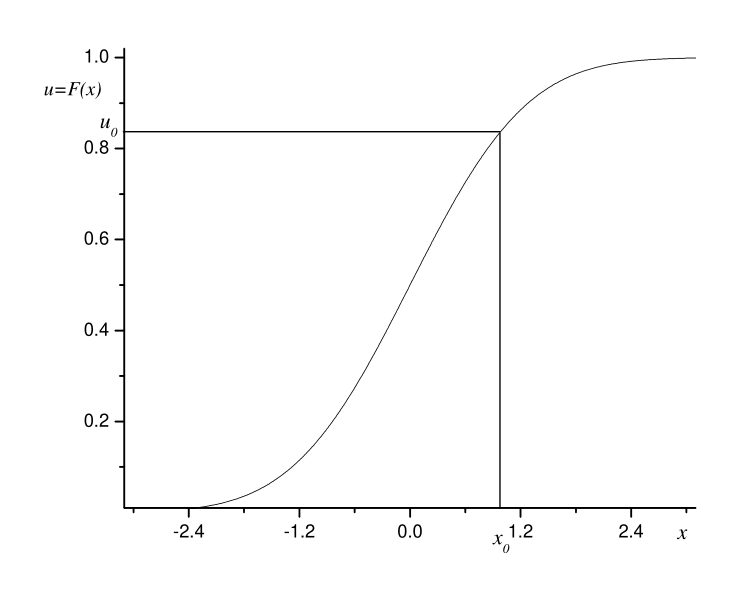
In Figure 3.1, we illustrate how to generate a realization of a random variable \(X\) with density \(f\) and cumulative distribution function \(F\). Thus, it suffices to generate a uniform random number \(u_0\) and invert the distribution function \(F\) at that point. Computationally, the difficulty lies in analytically deriving an expression for \(F^{-1}\) for many probability models. In general, closed-form expressions do not exist, and numerical methods are required to invert the distribution function. In this chapter, we present this method for the exponential distribution.
Figure 3.1: Illustration of the fundamental probability integral transform theorem for generating a random variable \(X\) with density \(f(x)=F'(x)\). Starting from a uniform random number \(u_0\), the distribution function is inverted at that point to obtain \(x_0\), with density \(f(x)\).
Another very general method that we will use is the rejection sampling method. This method has strong geometric appeal. We will first describe it in a broad, general manner. Later, we will apply it to generate random variables from specific probability models. The main advantage of this method is that it does not require computing the cumulative distribution function nor its inverse. These strategies can only be applied to many existing probability models if iterative numerical methods are used. Let \(f(x)\) be the probability density function from which we want to generate a random sample. The area under the curve over any interval of \(x\) corresponds to the probability of generating a value \(x\) in that interval. If we could generate a two-dimensional point, say \((X,Y)\), uniformly distributed over the area under the curve, then the \(X\)-coordinate would follow the target distribution.
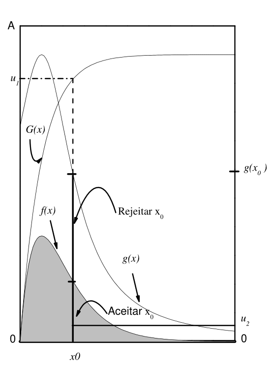
To efficiently generate realizations of random variables with density \(f(x)\) while avoiding the aforementioned numerical complications, we can define an arbitrary function \(g(x)\). This function must satisfy specific properties: it must have finite area and, for all \(x\), its values \(g(x)\) must be greater than or equal to \(f(x)\). This function is called a majorizing function (or comparison function). Another important property of \(g(x)\) is that its distribution function \(G(x)\) must be analytically computable and invertible, i.e., \(x=G^{-1}(u)\). Since \(g(x)\) is not necessarily a valid density function, let us denote the total area under this curve over the domain of interest as \(A=\int_{-\infty}^{\infty}g(x)dx\). Since \(G^{-1}\) is known, we can easily generate uniform points \((x,y)\) lying under the curve \(g(x)\). To do so, we generate a uniform random variable \(u_1\) between \(0\) and \(A\) and apply Theorem 3.1. This yields the first coordinate \(x_0=G^{-1}(u_1)\). To generate the second coordinate, we cannot simply draw a uniform variable on \([0, A]\), as that might produce a point outside the curve \(g(x)\). Instead, we evaluate \(g\) at \(x_0\), obtaining \(g(x_0)\), and draw \(y_0=u_2\), where \(u_2\) is a uniform random variable on \([0, g(x_0)]\). This yields a point \((x_0,y_0)\) uniformly distributed under the curve \(g(x)\). The challenge of this method lies precisely in defining a majorizing function \(g(x)\) that satisfies these required properties.
Now, let us plot the curves corresponding to \(g(x)\) and \(f(x)\) on the same graph. If the uniform point \((x_0,y_0)\) falls within the area under \(f(x)\)—that is, if \(y_0 \le f(x_0)\)—we accept \(x_0\) as a valid realization from \(f(x)\). If, on the other hand, the point lies in the region between \(f(x)\) and \(g(x)\)—that is, if \(f(x_0)<y_0 \le g(x_0)\)—we reject \(x_0\). An alternative way to express this criterion is to draw \(y_0\) from a \(U(0, 1)\) distribution and accept or reject \(x_0\) depending on whether \(y_0 \le f(x_0)/g(x_0)\) or \(y_0 > f(x_0)/g(x_0)\), respectively. We illustrate this method in Figure 3.2, where \(A\) represents the total area under \(g(x)\).
Figure 3.2: Rejection method for generating a value \(x_0\) of a random variable \(X\) with density function \(f(x)\) that is majorized by \(g(x)\) for all \(x\). In this illustration, \(x_0\) should be accepted.
Let us illustrate the first method and note that the second method is the one most commonly encountered in random variable generation. The exponential distribution is a probability distribution to which we can easily apply Theorem 3.1 to generate random samples. We choose to start the random variable generation process with this distribution because its distribution function and inverse are straightforward to obtain analytically. Let \(X\) be a random variable whose exponential density is given by:
\[f(x)=\lambda e^{-\lambda x} \tag{3.1}\]
where \(\lambda>0\) is the rate parameter of the exponential distribution and \(x>0\).
The exponential cumulative distribution function is given by:
\[F(x)=1-e^{-\lambda x} \tag{3.2}\]
The inverse cumulative distribution function \(x=F^{-1}(u)\) is given by:
where \(u\) is a uniform random number in \((0, 1)\).
Since the uniform distribution is symmetric on \((0,1)\), we can replace \(1-u\) in equation (3.3) with \(u\). Thus, to generate a realization of an exponential random variable \(X\) from a uniform random variable, we apply Theorem 3.1 via the expression:
\[x=\frac{-\ln(u)}{\lambda} \tag{3.4}\]
The Python algorithm to generate realizations of exponential random variables is:
We can use Python’s built-in function (np.random.exponential(scale=1.0, size=None)) to accomplish the same task. Simply typing np.random.exponential(scale=10, size=5) produces a random sample of size \(n\) from an exponential distribution with parameter \(\lambda=1/\textrm{scale}\). Python makes computational statistics straightforward and accessible to researchers.
3.3 Random Variables from Important Distributions
In this section, we describe specific methods for generating realizations of several key random variables, with emphasis on the normal distribution. Although the general method presented in Section 3.2 can also be applied to the normal distribution, we focus on alternative procedures. To use the inversion method, we would need a function similar to rexpon, say rnormal. In place of x = -log(u)/lamb, we would write \(x=\textrm{invnorm}(u)\times\sigma + \mu\), where invnorm(u) is the inverse cumulative distribution function of the standard normal distribution. The standard normal distribution within the normal family—defined by parameters \(\mu\) and \(\sigma^2\)—is the one with zero mean and unit variance, denoted by \(N(0, 1)\). This inverse function would need to be written externally by the user. The parameters \(\mu\) and \(\sigma\) passed to the function are the mean and standard deviation of the target normal distribution. The normal probability density function is:
We will not present additional functions relying directly on Theorem 3.1, as one can easily adapt functions like rexpon given an efficient algorithm for inverting the cumulative distribution function of the target model. The drawback of this approach is the substantial computational effort required for most densities, which can lead to high execution times and algorithmic inefficiency.
Furthermore, we can leverage relationships between probability distributions to generate realizations from other distributions. For example, if \(X\) is normal with density (3.5), \(N(\mu,\sigma^2)\), we can generate realizations of \(Y=e^X\). Under this transformation, \(Y\) follows a log-normal distribution with location parameter \(\alpha\) (\(\mu\)) and scale parameter \(\beta\) (\(\sigma\)), whose density function is:
An important algorithm used to generate normal variates is the Box-Muller method, which is based on generalizing the variable transformation technique to higher dimensions. To present this method, consider \(p\) random variables \(X_1, X_2, \ldots, X_p\) with joint density function \(f(x_1, x_2, \ldots, x_p)\) and \(p\) variables \(Y_1, Y_2, \ldots, Y_p\) that are functions of all \(X\)’s. The joint probability density function of the \(Y\)’s is:
where \(J=\left| \partial()/\partial()\right|\) is the Jacobian of the transformation from the \(X\)’s to the \(Y\)’s.
Let us apply transformation (3.7) to generate normal data with density given by (3.5). For the Box-Muller transformation, consider two uniform random variables on \([0, 1]\), denoted \(X_1\) and \(X_2\), and two functions \(Y_1\) and \(Y_2\) defined by:
Using the derivative rule \(\frac{d}{dx}[k\arctan(g)] = \frac{k g'}{1+g^2}\), where \(g\) is a function of \(x\), the Jacobian matrix of the transformation is:
Since the joint density of \(Y_1\) and \(Y_2\) is the product of two independent normal densities, \(Y_1\) and \(Y_2\) are independent standard normal random variables, as shown in Johnson and Wichern (1998) and Ferreira (2018).
Thus, we can use this result to generate normal random variables. The main drawback is computational: evaluating trigonometric functions such as sine and cosine can slow down the algorithm. A clever modification proposed by Marsaglia and Bray (1964) (and detailed in Press et al. (1992)) avoids direct evaluation of trigonometric functions. This variant is known as the Polar Box-Muller method.
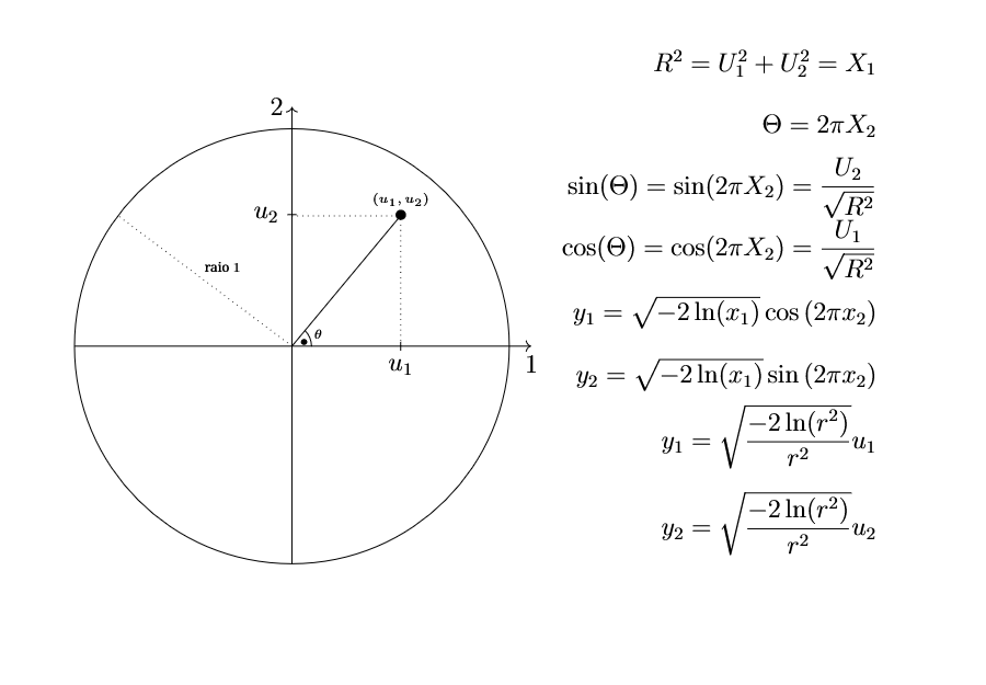
Instead of selecting uniform random variables \(x_1\) and \(x_2\) from a unit square, we sample points \((u_1, u_2)\) uniformly distributed inside a unit circle (radius \(1\)). The sum of their squares, \(R^2=U_1^2+U_2^2\), is a uniform random variable that can serve as \(X_1\), while the angle \(\Theta\) formed by \((u_1, u_2)\) relative to the horizontal axis serves as the random angle \(\Theta=2\pi X_2\). The key advantage of avoiding expression (3.8) directly is that cosine and sine can be obtained algebraically: \(\cos{(2\pi x_2)}=u_1/\sqrt{r^2}\) and \(\sin{(2\pi x_2)}=u_2/\sqrt{r^2}\). This eliminates trigonometric function calls. In Figure 3.3, we illustrate these concepts, denoting the angle between \((u_1,u_2)\) and the \(u_1\)-axis as \(\theta\).
Figure 3.3: Unit circle showing a random point \((u_1, u_2)\) with \(r^2 = u_1^2 + u_2^2\) representing \(x_1\) and \(\theta\) representing the angle formed by \((u_1, u_2)\) relative to the horizontal axis. In this illustration, the point lies inside the unit circle as required.
Now we present the boxmuller function to generate normal random variables using the Polar Box-Muller algorithm. This function relies on an inner helper polar to generate two independent standard normal variates \(Y_1\) and \(Y_2\):
Several approximations are outlined in Atkinson and Pearce (1976) and summarized below. One approximation relies on the Tukey-lambda distribution, fitting a normal curve by matching the first four moments. In addition to being an approximation, this method suffers from the computational expense of exponentiation. Using this approximation, a normal variable \(X\) can be generated from a uniform variable \(U \sim U(0, 1)\) via:
Another approximation is based on summing \(12\) or more independent uniform variables (\(U_i \sim U(0, 1)\)). By the Central Limit Theorem, the variable \(X=\sum_{i=1}^{12} U_i - 6\) is approximately standard normal \(N(0, 1)\), because each of the \(12\) uniform variables has mean \(1/2\) and variance \(1/12\).
These two approximations have primarily pedagogical value and are not recommended for production applications requiring high precision. In practice, relying on coarse approximations can yield inaccurate or misleading conclusions.
In general, summing \(k\) uniform variables yields:
since \(E(U_i)=(b-a)/2\) and \(V(U_i)=(b-a)^2/12\), where \(k\) is the number of uniform variables summed per normal realization. Below, we implement both approximations in Python as instructional exercises.
The first is the Tukey-Lambda approximation:
The second is the sum of \(k\) uniform variables via the Central Limit Theorem:
We can also implement a vectorized version of this CLT approximation (analogous to using apply in R), as shown in the script below:
3.4 Binomial Distribution
We now move to discrete distributions, illustrating random variable generation with the binomial model. The binomial distribution plays a central role in applied statistics across diverse empirical contexts. For instance, the non-parametric sign test relies on the binomial distribution, and the count of diseased animals in a random sample of size \(n\) is frequently modeled binomially. A random variable \(X\) following a binomial distribution has probability mass function given by:
\[P(X=x)= \binom{n}{x} p^x(1-p)^{n-x}, \qquad x=0, 1,\cdots, n \quad \textrm{and} \quad n \ge 1 \tag{3.12}\]
where the parameters \(n\) and \(p\) denote the number of trials and the success probability per trial, respectively. The term \(\binom{n}{x}\) is the binomial coefficient:
The probability of success \(p\) must remain constant across the \(n\) independent Bernoulli trials. The parameter \(n\) is specified by the researcher as an integer \(n \ge 1\). When \(n=1\), the binomial distribution reduces to a Bernoulli distribution. Thus, a binomial variable represents the total number of successes in \(n\) independent, identically distributed Bernoulli trials. The following theorems and lemmas underpin the generation algorithms presented below.
Theorem 3.2 (Genesis) Let \(X\) be the number of successes in a sequence of \(n\) Bernoulli trials with success probability \(p\), i.e., \[X=\sum_{i=1}^{n}I(U_i \le p)\] where \(U_1, U_2, \dots, U_n\) are i.i.d. uniform random variables \(U(0, 1)\) and \(I(\bullet)\) is an indicator function. Then \(X\) follows a binomial distribution \((n, p)\).
Lemma 3.1 (Sum of Binomials) If \(X_1, X_2, \dots, X_k\) are independent binomial random variables with parameters \((n_1, p), \dots, (n_k, p)\), then \(\sum_{i=1}^{k} X_i\) follows a binomial distribution with parameters \((\sum_{i=1}^{k}n_i, p)\).
Lemma 3.2 (Waiting Time - Property 1) Let \(G_1, G_2, \dots\) be independent geometric random variables, and let \(X\) be the smallest integer such that \[\sum_{i=1}^{X+1} G_i > n.\] Then \(X\) follows a binomial distribution \((n, p)\).
The geometric variables in Lemma 3.2 are defined as follows: if \(G\) follows a geometric distribution with constant success probability \(p \in (0, 1)\), its probability mass function is:
The geometric distribution models the waiting time (trial number) until the first success in a sequence of independent Bernoulli trials. It assumes \(g-1\) failures (each with probability \(1-p\)) preceding a success on the \(g\)-th trial (with probability \(p\)). The second waiting time lemma is stated below:
Lemma 3.3 (Waiting Time - Property 2) Let \(E_1, E_2, \dots\) be i.i.d. exponential random variables, and let \(X\) be the smallest integer such that \[\sum_{i=1}^{X+1} \frac{E_i}{n-i+1} > -\ln(1-p).\] Then \(X\) follows a binomial distribution \((n, p)\).
These theoretical properties form the foundation for several binomial sampling algorithms. The most basic binomial algorithm generates \(n\) independent \(U(0, 1)\) variables and counts how many are \(\le p\). This algorithm, designated BU by Kachitvichyanukul and Schmeiser (1988), proceeds as follows:
Set \(x=0\) and \(k=0\);
Generate \(u \sim U(0, 1)\) and set \(k=k+1\);
If \(u \le p\), set \(x=x+1\);
If \(k<n\), return to step 2;
Return \(x\) as a draw from a binomial \((n, p)\).
The BU algorithm has execution speed proportional to \(n\) and depends on the speed of the underlying uniform generator, but it requires no setup variables. Its Python implementation is:
A second algorithm, developed by Devroye (1980) (Devroye 1980) and named BG, is based on Lemma 3.2. The BG algorithm works as follows:
Set \(y=0\), \(x=0\), and \(c=\ln(1-p)\);
If \(c = 0\), skip to step 6;
Generate \(u \sim U(0, 1)\);
Set \(y=y+\lfloor \ln(u)/c \rfloor+1\), where \(\lfloor \bullet \rfloor\) denotes the floor function;
If \(y \le n\), set \(x=x+1\) and return to step 3;
Return \(x\) as a draw from a binomial \((n, p)\).
In step 4 of algorithm BG, a geometric random variable is generated by truncating an exponential variable, \(G=\lfloor \ln(U)/c \rfloor+1 \sim G(p)\), as described by Devroye (1986). The execution time of this algorithm is proportional to \(n \cdot p\), representing a substantial performance improvement. When \(p > 0.5\), we can optimize BG further by exploiting the symmetry property: if \(X \sim \text{Binomial}(n, p)\), then \(n-X \sim \text{Binomial}(n, 1-p)\). We replace \(p\) with \(\min(p, 1-p)\) and return \(x\) if \(p \le 0.5\), or \(n-x\) otherwise. The overall speed is thus proportional to \(n \cdot \min(p, 1-p)\).
A disadvantage of algorithm BG is that multiple uniform random numbers may be drawn before returning a single binomial value \(x\). An alternative approach is to use an inversion algorithm based on the discrete distribution function.
As noted previously, the inversion method is the standard approach for converting a uniform variable \(U\) into a random variable \(X\) by inverting \(F\). For continuous variables, the steps are:
Generate uniform \(u \sim U(0,1)\)
Return \(x=F^{-1}(u)\)
For discrete variables, inversion requires searching for the integer value \(x\) such that:
The simplest search strategy is a sequential search starting at \(x=0\). For the binomial distribution, this inversion algorithm—designated BINV—uses the recursive recurrence relation:
for \(x=1, 2, \dots, n\) through the following steps:
Set \(pp=\min(p, 1-p)\), \(qq=1-pp\), \(r = pp / qq\), \(g=r(n+1)\), and \(f=qq^n\);
Generate \(u \sim U(0, 1)\), set \(x=0\), and set \(F=f\);
If \(F \ge u\), skip to step 5;
Set \(x = x + 1\), \(f=f\left(\dfrac{g}{x}-r\right)\), \(F=F + f\), and return to step 3;
If \(p \le 0.5\), return \(x\); otherwise return \(n-x\).
The speed of this algorithm is proportional to \(n \cdot \min(p, 1-p)\). Its advantage is that only a single uniform variable is drawn per binomial realization. However, computing \(qq^n\) can be computationally expensive, and two potential numerical issues may arise: (i) numerical underflow when computing \(f=qq^n\) for large \(n\), and (ii) accumulation of round-off errors during recursive updates of \(f\) as \(n\) grows (Kachitvichyanukul and Schmeiser 1988). Devroye (1986) suggests using the waiting-time algorithm BG based on Lemma 3.2 instead of BINV to avoid these issues. On the other hand, Kachitvichyanukul and Schmeiser (1988) note that double-precision arithmetic effectively mitigates these precision concerns.
We can implement a parallelized version of BG using Numba (pip install numba). While vectorizing BG directly is difficult due to the random number of while loop iterations, Numba provides a straightforward alternative. Numba compiles pure Python loop constructs into machine code, enabling native parallelization across CPU cores via prange (parallel range). The prange construct informs Numba’s compiler that iterations of the loop are mutually independent.
Combining prange with parallel=True allows Numba to automatically distribute \(n\) simulations across available CPU threads. The @njit decorator (short for no-Python mode JIT) compiles Python code into native machine code assembly, bypassing the Python interpreter entirely. If desired, the thread count can be fixed explicitly via numba.set_num_threads(k). In the script below, this call is commented out, allowing Numba to utilize all available CPU cores.
The following code illustrates this implementation:
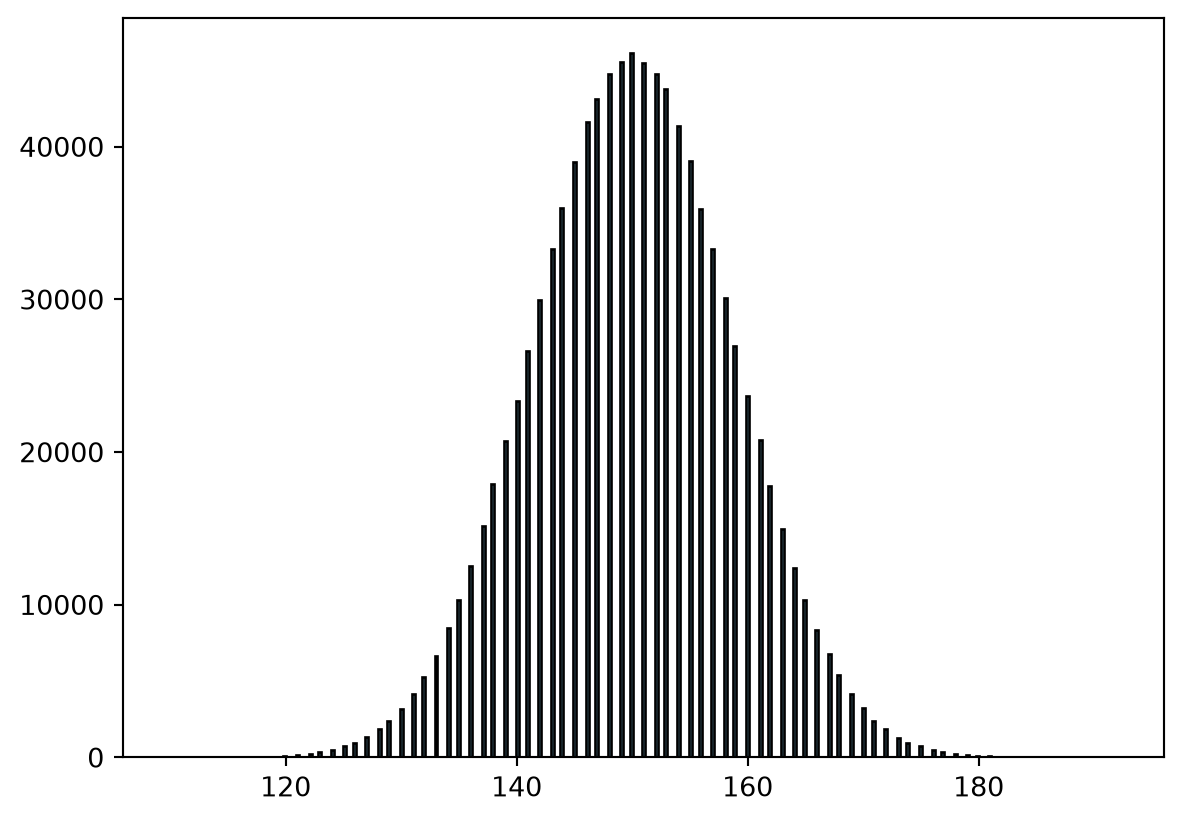
import numpy as npimport matplotlib.pyplot as pltfrom numba import njit, prange# Explicitly set the number of CPU threads used by Numba# numba.set_num_threads(4) @njit# Compiles the function for C-like execution speeddef bg_single(size, p): pp =1- p if p >0.5else p y, x =0, 0 c = np.log(1- pp)if c <0:while y <= size: u = np.random.uniform(0.0, 1.0) y +=int(np.trunc(np.log(u) / c) +1)if y <= size: x +=1if p >0.5: x = size - xreturn x@njit(parallel=True) # Runs simulations in parallel across CPU coresdef rbinom_bg_numba(n, size, p): out = np.empty(n, dtype=np.int64)for i in prange(n): out[i] = bg_single(size, p)return out# Usage example:n =1000000size =300p =0.5x = rbinom_bg_numba(n, size, p)# Create an isolated space for the figurefig, ax = plt.subplots()# Draw the histogram_ = ax.hist(x, bins=size +1, rwidth=0.95, edgecolor='black', color='skyblue')# Display the plot nativelyplt.show()
WarningPyodide Limitations (Numba and Memory Constraints)
Pyodide executes Python inside WebAssembly (WASM) within the browser environment, imposing strict operational limits:
Incompatibility with Numba: Numba requires LLVM to generate native machine code dynamically (JIT). Because Pyodide operates within a browser sandbox, dynamic JIT compilation is unsupported. Remove or comment out decorators like @jit or @njit.
32-bit Memory Model: WASM uses 32-bit memory addressing by default, constraining available heap space.
2 GB to 4 GB Maximum Memory Limit: Even if your physical system has 16 GB or 32 GB of RAM, Pyodide allocates a maximum of 2 GB to 4 GB for the entire Python session. Operations requesting large contiguous NumPy arrays can easily exceed this limit.
Conversely, for the BU method, a vectorized array implementation can be constructed as follows to generate samples of size \(n\):
The command np.random.uniform(size=(n, size)) creates an \(n \times \text{size}\) matrix of uniform random numbers. The expression (u <= prob).sum(axis=1) evaluates to a boolean matrix of True/False values and sums True (=1) entries across columns for each of the \(n\) rows. These two vectorized adaptations significantly boost computational efficiency.
While random number generators can be developed manually for many other distributions, Python provides optimized, pre-compiled routines for standard probability models in lower-level compiled code. We cover these built-in routines in the next section.
3.5 Python Routines for Generating Random Variables
In this section, we review the primary Python functions used to generate random variables from common probability distributions. The probability models supported by NumPy are summarized in Table 3.1.
Table 3.1: Probability distributions, NumPy function names (np.random.col2name), and arguments, where size specifies the output sample size.
Distribution
NumPy Name
Parameters
Beta
beta(a, b, size=None)
a, b, size
Binomial
binomial(n, p, size=None)
n, p, size
Standard Cauchy
standard_cauchy(size=None)
size
Chi-Square
chisquare(df, size=None)
df, size
Exponential
exponential(scale=1.0, size=None)
scale (1/lambda), size
F
f(dfnum, dfden, size=None)
dfnum, dfden, size
Gamma
gamma(shape, scale=1.0, size=None)
shape, scale (1/beta), size
Geometric
geometric(p, size=None)
p, size
Hypergeometric
hypergeometric(ngood, nbad, nsample, size=None)
ngood, nbad, nsample, size
Log-Normal
lognormal(mean=0.0, sigma=1.0, size=None)
mean, sigma, size
Logistic
logistic(loc=0.0, scale=1.0, size=None)
loc, scale, size
Negative Binomial
negative_binomial(n, p, size=None)
n, p, size
Normal
normal(loc=0.0, scale=1.0, size=None)
loc, scale, size
Poisson
poisson(lam=1.0, size=None)
lam, size
Student’s t
standard_t(df, size=None)
df, size
Uniform
uniform(low=0.0, high=1.0, size=None)
low, high, size
Weibull
weibull(a, size=None)
a, size
In Python, the scipy.stats module enables evaluation of probability mass functions (discrete distributions) via functions like sp.stats.binom.pmf(x, n, p), where sp represents scipy and pmf stands for Probability Mass Function. For continuous distributions, the corresponding method is pdf (Probability Density Function). Cumulative distribution functions are evaluated via cdf for both continuous and discrete models, while inverse cumulative distribution functions use ppf (Percent Point Function), which takes accumulated probability as its primary argument. Non-central distribution variants are also supported via non-centrality parameters (ncp). Additional information is available in the official scipy.stats documentation.
Using these routines to sample random variables is straightforward. For instance, to sample from a Beta distribution with parameters \(\alpha=1\) and \(\beta=2\), we can execute the following code script. Similar NumPy routines listed in Table 3.1 can generate samples of size \(n\) for other probability density or mass functions. Built-in functions are significantly faster than pure Python implementations because they execute optimized C code. If custom distributions must be sampled millions of times, compiling C routines and binding them to Python offers optimal performance.
3.6 Exercises
Let \(f(x)=3x^2\) be the probability density function of a continuous random variable \(X\) defined on \([0, 1]\). Apply the inversion method to derive an algorithm for generating random variables from this density. Implement the algorithm in Python and generate a sample of size \(n=1,000\). Estimate the \(1\%\), \(5\%\), \(10\%\), \(50\%\), \(90\%\), \(95\%\), and \(99\%\) quantiles and compare them against theoretical quantiles.
Use Numba to parallelize the Polar Box-Muller method and improve its efficiency. Compare execution speed against the original pure Python implementation and NumPy.
The dataset below contains the lifespan (in days) of \(n=40\) insects. Assuming lifespan follows an exponential distribution where the rate parameter \(\lambda\) is estimated by the maximum likelihood estimator \(\hat{\lambda}=1/\bar{X}\) (\(\bar{X}=\sum_{i=1}^{n}X_i/n\)), obtain a \(95\%\) confidence interval using the following parametric bootstrap procedure: (i) generate a sample of size \(n=40\) from an exponential distribution using np.random.exponential with parameter equal to the estimated rate; (ii) calculate the sample mean \(\bar{X}\) to estimate \(\mu=1/\lambda\); (iii) repeat steps (i) and (ii) \(1,000\) times and store the resulting estimates; (iv) sort the estimates and extract the \(2.5\%\) and \(97.5\%\) quantiles. The recorded lifespans (in days) are:
8.521
4.187
2.516
1.913
8.780
5.912
0.761
12.037
2.604
1.689
5.626
6.361
5.068
3.031
1.128
1.385
12.578
2.029
0.595
0.445
3.601
7.829
1.383
1.934
0.864
8.514
4.977
0.576
1.503
0.475
1.041
0.301
1.781
2.564
5.359
2.307
1.530
8.105
3.151
8.628
Repeat this procedure using \(100,000\) bootstrap replicates of size \(n=40\). Compare results and evaluate whether the additional computational cost of increasing bootstrap replicates produced a meaningful gain in precision.
Generate a sample of \(n=5,000\) standard normal realizations using two approximations: (a) \(X=[U^{0.135} - (1-U)^{0.135}] / 0.1975\) and (b) the sum of \(12\) independent uniform variables \(X=\sum_{i=1}^{12} U_i - 6\). Compare the empirical \(1\%\), \(5\%\), \(10\%\), \(50\%\), \(90\%\), \(95\%\), and \(99\%\) quantiles against theoretical standard normal quantiles. Generate an additional sample of size \(n=5,000\) using the Polar Box-Muller algorithm, calculate the same sample quantiles, and compare across all methods.
Assuming the insect lifespan dataset from Exercise 3 can be modeled by a log-normal distribution, estimate the log-normal parameters and apply the parametric bootstrap approach to construct a confidence interval for the population mean. To estimate log-normal parameters: (a) log-transform the original data, \(X^*_i = \ln(X_i)\); (b) calculate the sample mean and standard deviation of \(X^*_i\), using these as estimates for \(\mu\) and \(\sigma\). Use these parameters to generate log-normal samples by drawing standard normal variates \(Z \sim N(0, 1)\), transforming to \(Y = S Z + \bar{X}\), and setting \(X = \exp(Y)\). Perform the bootstrap procedure, compare results against the exponential model, and discuss the challenges of selecting an underlying probability model for statistical inference. How might one empirically determine which probability distribution best fits the insect lifespan data? Justify your answer using appropriate statistical and numerical criteria.
Perform non-parametric bootstrap resampling with replacement from the sample in Exercise 3 to estimate a \(95\%\) confidence interval for the population mean, using a uniform random generator to select bootstrap sample indices: (i) resample \(n=40\) observations with replacement from the original dataset to form \(X^*_i\); (ii) compute the bootstrap sample mean \(\bar{X}^* = \sum_{i=1}^{n} X_i^*/n\); (iii) record this mean and repeat steps (i) and (ii) \(B-1\) times; (iv) combine the bootstrap estimates with the original sample mean; and (v) sort the values and extract the \(2.5\%\) and \(97.5\%\) quantiles across all \(B\) values. Perform the procedure for \(B=1,000\) and \(B=100,000\), comparing the resulting confidence bounds with those obtained for the exponential and log-normal models in previous exercises. Models yielding confidence bounds closest to the non-parametric bootstrap provide empirical evidence regarding distribution fit. Discuss the primary advantage of non-parametric bootstrapping in avoiding distribution assumptions.
A fundamental property of the exponential distribution, \(f(x) = \lambda e^{-\lambda x}\), is that the sum of \(n\) independent and identically distributed (i.i.d.) random variables \(X_i \sim \text{Exp}(\lambda)\) follows a Gamma distribution with shape parameter \(\alpha = n\) and scale parameter \(\beta = 1/\lambda\):
with \(\alpha = n\). This property allows us to avoid drawing \(n\) individual random variates across each of the \(B\) parametric bootstrap replicates. Assuming the data in Exercise 3 follow an exponential distribution, we can estimate the population scale parameter \(\beta\) using the sample mean, \(\hat{\beta} = \bar{X}\). Using this estimator, implement an optimized parametric bootstrap that directly simulates the sample mean distribution (\(\bar{Y}\)) via the following steps:
(i) Draw a vector of size $B$ directly from a **Standard Gamma** distribution ($\alpha = n$, scale $\beta = 1$) to model the stochastic structure of the sum;
(ii) Scale the sums by multiplying by $\hat{\beta}$ (i.e., $Y = \hat{\beta} \cdot \text{Standard Gamma}$);
(iii) Divide by sample size $n$ to obtain simulated sample means: $\bar{Y} = Y / n$;
(iv) Sort the resulting values and extract the $2.5\%$ and $97.5\%$ quantiles to construct a $95\%$ confidence interval. Perform simulations for $B = 1,000$ and $B = 100,000$, compare numerical results against Exercise 3, and answer:

- **(a)** What conclusions can be drawn regarding the confidence interval bounds produced by both strategies?
- **(b)** What are the key computational advantages (in terms of memory usage and processing time) of sampling from the Gamma distribution directly compared to generating full samples of size $n$?
Two binomial samples were collected from two distinct populations (\(1\) and \(2\)). The observed success counts were \(y_1=2\) and \(y_2=3\) in samples of size \(n_1=12\) and \(n_2=14\), respectively. Estimate population parameters \(p_1\) and \(p_2\) using sample proportions \(\hat{p}_1=y_1/n_1\) and \(\hat{p}_2=y_2/n_2\). To test the hypothesis \(H_0: p_1=p_2\) (or \(H_0: p_1-p_2 = 0\)), implement the following parametric bootstrap algorithm: (a) use \(\hat{p}_1\) and \(\hat{p}_2\) to generate binomial samples of size \(n_1\) and \(n_2\) from both populations; (b) compute bootstrap estimates \(\hat{p}_{1j}=y_{1j}/n_1\) and \(\hat{p}_{2j}=y_{2j}/n_2\) on iteration \(j\); (c) calculate \(d_j=\hat{p}_{1j}-\hat{p}_{2j}\); (d) repeat steps (a) through (c) \(B-1\) times; (e) combine bootstrap difference estimates with the original sample difference; (f) sort the values and extract the \(2.5\%\) and \(97.5\%\) quantiles of the bootstrap distribution of \(d_j\); and (g) if \(0\) lies within this confidence interval, do not reject \(H_0\); otherwise, reject \(H_0\) in favor of unequal population proportions.
Atkinson, A. C., and M. C. Pearce. 1976. “The Computer Generation of Beta, Gamma and Normal Random Variable.”Journal of the Royal Statistical Society, Series A 139 (4): 431–61.
Devroye, L. 1980. “Generating the Maximum of Independent Identically Distributed Random Variables.”Computers and Mathematics with Applications 6: 305–15.
Devroye, L. 1986. Non-Uniform Random Variate Generation. Springer-Verlag.
Ferreira, Daniel Furtado. 2018. Estatística Multivariada. 3rd ed. Editora UFLA.
Johnson, R. A., and D. W. Wichern. 1998. Applied Multivariate Statistical Analysis. 4th ed. Prentice Hall.
Kachitvichyanukul, V., and B. W. Schmeiser. 1988. “Binomial Random Variate Generation.”Communications of the ACM 31 (2): 216–22.
Marsaglia, G., and T. A. Bray. 1964. “A Convenient Method for Generating Normal Variables.”SIAM Review 6 (3): 260–64.
Press, W. H., B. P. Flannery, S. A. Teukolsky, and W. T. Vetterling. 1992. Numerical Recipes in Fortran: The Art of Scientific Computing. Cambridge University Press.