6 Approximation of Distributions
Algorithms for obtaining probabilities have been the subject of research for many decades and still are. The importance of having algorithms that are both fast and accurate is indescribable. The main difficulty is that most probabilistic models do not have an explicitly known distribution function. Thus, sophisticated numerical methods are required to compute probabilities. Another aspect is the need to invert distribution functions to obtain quantiles of the random variable for a known cumulative probability. In hypothesis tests and in interval and region estimation procedures, we almost always use these algorithms indirectly without realizing it.
In this chapter, we will introduce these concepts and present some basic ideas of general methods for performing the necessary quadratures. Particular numerical methods will be addressed for a few models. We will also address the discrete and continuous cases separately. To conclude, we will present the main pre-existing Python functions for a series of probabilistic models.
6.1 Introduction
We do not have many concerns about obtaining probabilities and quantiles when using Python, since most probabilistic models and special functions are already implemented. Our objective goes beyond this fact, as our intention is to seek the knowledge necessary to go further and to understand how a given function operates and what its capabilities and limitations are.
We will begin our discussion with the exponential distribution to draw attention to the main difficulty in this process. Thus, we chose this model precisely because it does not present such difficulties. Considering a random variable \(X\) with exponential distribution with parameter \(\lambda\), we have the density function \[ f(x) = \lambda e^{-\lambda x}, \quad x>0 \tag{6.1}\] and the distribution function \[ F(x)=1-e^{-\lambda x}. \tag{6.2}\]
For this probabilistic model, we can compute probabilities using the distribution function (6.2) and obtain quantiles with the inverse distribution function given by: \[ q=F^{-1}(p)=\dfrac{-\ln(1-p)}{\lambda}. \tag{6.3}\]
We implemented, in Python, the density, distribution, and inverse distribution functions and named them dexp, pexp, and qexp, respectively. These functions are:
In the case where the user enters scalar values (integers or float) or lists of values, the previous functions convert them into NumPy lists using the stacked methods np.atleast_1d(np.asarray(x, dtype=float)) and np.atleast_1d(np.asarray(p, dtype=float)). If the argument is a scalar, the np.asarray method converts it into a 0-dimensional array of float type, and the other method, np.atleast_1d, converts it into an array with at least one dimension (NumPy list). The advantage of this conversion method is that it does not create additional copies of the argument in memory if it is already a list. The other method, which we will present in the next function, is np.array(x, ndmin=1, dtype=float), which performs the same conversion much more quickly but duplicates the variable x in memory. The ndmin=1 option ensures that the number of dimensions of the created float array is at least 1. In some cases, efficiency in terms of processing speed should be chosen; in others, memory efficiency is the right option.
Another concern we should have is regarding possible incorrect user inputs in the function arguments. We have not had many concerns so far about possible errors in calls to our functions with incorrect arguments. To illustrate, let us consider only the exponential probability density function. In this case, if \(\lambda>0\) and the values of \(x\) are positive or zero, we have no problem. If, on the other hand, the values of \(x\) are negative, then the density value should be zero. This kind of concern existed in the implementation of the previous dexp function. However, we may have zero or negative values of the parameter \(\lambda\) used incorrectly in the function call, which is not a valid procedure, and no protection against this action was made. Thus, it is prudent that some problems be anticipated and consistent results be returned. In this case, the result nan should be returned, since the density function is not valid under these conditions. Furthermore, the lamb argument of the function is considered a scalar, but the x argument can be a vector. We can also handle this case by treating both arguments as vectors, even if we do not change the scalar value of the default lamb argument, and by adjusting their dimensions if they have different sizes. The following program illustrates this and uses np.resize to perform this adjustment.
In this case, this function automatically resizes the vectors by repetition to equalize their sizes before the element-wise computation. This occurs with the use of np.resize, after the maximum size relative to the sizes of both vectors is obtained. If the sizes are different, an incomplete recycling of the smaller vector is performed through cyclic repetition, truncating the result when it reaches the size of the larger vector, without completing the last cycle. This means that a cyclic recycling of the smaller vector is performed, interrupting the repetition when it reaches the exact size of the larger vector, even if this means leaving the last cycle incomplete. After adjusting the vector sizes, a result vector is created for the results with nan. Thus, if there are invalid values in the argument inputs, a combined boolean mask of non-negative x values and zero or positive lamb values is obtained. The density is computed only where these two conditions occur simultaneously, and the nan values of result are replaced by the density values. The problem is that if x is negative and lamb is positive, the density value should be zero and is not computed using the previous mask. But if x is negative and lambda is invalid, the previously defined nan values in result are kept. By definition, the probability density function exists for all reals, provided that the model parameters are correctly defined. The program makes a specific final adjustment for the case where x is negative but lamb is positive, with the command result[(x_expanded < 0) & valid_lambda] = 0.0 (see case 6).
The Python functions for the exponential were easily implemented, since we can explicitly obtain the distribution function and its inverse. If, on the other hand, we had the normal model \[ f(x) = \dfrac{1}{\sqrt{2\pi\sigma^2}} \exp\left\{-\dfrac{(x-\mu)^2}{2\sigma^2}\right\} \tag{6.4}\] we could not explicitly obtain the distribution function, much less the inverse of the probability distribution function. Since for the vast majority of probabilistic models we encounter the same problems, we need numerical methods to obtain these functions. For this reason, we will present some details in this chapter about some general and specific methods for certain models. In the discrete case, we can use sequential recursive algorithms. However, since most discrete probabilistic models have an exact relationship with continuous models, we encounter the same problems when using these relationships.
6.2 Discrete Probabilistic Models
We will present algorithms for obtaining the probability function, the probability distribution function, and its inverse for the discrete models we consider most important: the binomial and Poisson models. We will begin our discussion with the binomial model. Considering a random variable \(X\) with binomial distribution, its probability function is given by: \[ P(X=x) = \binom{n}{x} p^x (1-p)^{(n-x)} \tag{6.5}\] where \(n\) is the sample size or number of independent Bernoulli trials with success probability \(p\), and \(x\) is the number of successes, which belongs to the finite set \(0\), \(1\), \(\cdots\), \(n\). The probability distribution function is given by:
\[\begin{align}\label{apec6:eq:cdfbin} F(x) = & \sum_{t=0}^x \binom{n}{t} p^t (1-p)^{n-t}. \end{align}\]
We saw in chapter 3, equation (3.14), that we can obtain the cumulative probabilities recursively. Given \(P(X=0)= (1-p)^n\), we obtain the probabilities for the other values of \(X\), that is, for \(x=1\), \(\cdots\), \(n\), recursively using the relation \(P(X=x)=P(X=x-1)[(n-x+1)/x] [p/(1-p)]\). We can summarize it as follows: \[P(X=x)=P(X=x-1) \left(\dfrac{g}{x} - r\right),\] where \(r=p/(1-p)\) and \(g=r(n+1)\), for \(x=2\), \(3\), \(\cdots\), \(n\).
This same algorithm, appropriately modified, is used to obtain the cumulative probabilities and the inverse of the distribution function. If the values of \(n\) and \(p\) are large, this algorithm may be inefficient. For the case where the parameter \(p\) is large (close to one), we can use the binomial property given by: if \(X \sim\) \(Bin(n, p)\), then \(Y=n-X \sim\) \(Bin(n, 1-p)\). Thus, we can, for example, obtain \(P(X=x)\) equivalently by \(P(Y=n-x)\) and \(P(X\le x) = P(Y\ge n-x)\), which can be rewritten as \(F_X(x)= 1-F_Y(n-x-1)\), except for \(x=n\), where \(F_X(x)=1\). In this way, we switch variables to perform the computation and then return the value corresponding to the original event.
If we use the property that if \(X\) is binomial with parameters \(n\) and \(p\), then \(n-X\) is also binomial with parameters \(n\) and \(1-p\). Since the algorithm is more efficient when \(p<0.5\), because \(q\) \(=\) \(1-p\) is closer to \(1\) and the execution speed of the algorithm is proportional to \(np\). Thus, we gain processing time and precision if \(p>0.5\) and we perform the switch to \(n-X\). The following script presents this modification in the qbinom function:
The binomial distribution function has an exact relationship with the beta distribution function. If we have algorithms to obtain the incomplete beta, we can use this relationship to obtain probabilities of the binomial distribution. The binomial distribution function, \(F(x)\), relates to the incomplete beta function, \(Ip(\alpha,\beta)\), as follows:
\[ F(x;n,p) = \left\{ \begin{array}{ll} 1 - I_p(x+1,n-x), & \textrm{ if } 0\le x < n \\ 1, & \textrm{ if } x = n. \end{array} \right. \tag{6.6}\]
Thus, we can anticipate the importance of knowing numerical integration algorithms for continuous distributions. This becomes even more evident when we realize that for large values of \(n\) the recursive algorithms are inefficient and may become inaccurate. In Section 6.3 we will present some general integration methods for continuous functions. In the following script, we use relation (6.6) to obtain the binomial distribution function.
The Poisson distribution is the second one we will consider. There is a relationship between the Poisson distribution function and the incomplete gamma. If a discrete random variable \(X\) with values \(x=0\), \(1\), \(2\), \(3\), \(\cdots\) has a Poisson distribution with parameter \(\lambda\), then we can define the probability function as: \[ P(X=x) = \dfrac{\lambda^x e^{-\lambda}}{x!}. \tag{6.7}\]
We can obtain probabilities from this distribution using the relationship of the incomplete gamma with the Poisson distribution function \[
F(x|\lambda)=1-I_{\lambda}(\alpha=x+1), \qquad x=0, 1, 2, \cdots.
\tag{6.8}\] where \[\begin{align*}
I_{x}(\alpha)=\dfrac{1}{\Gamma(\alpha)}\int_0^x e^{-t}t^{\alpha-1}dt,
\end{align*}\] is the incomplete gamma function, for values of \(x\ge 0\). The script for this is
6.3 Continuous Probabilistic Models
To obtain the distribution function or the inverse of the distribution function of continuous probabilistic models, as a rule, we must use numerical methods. There are exceptions, such as the exponential model described at the beginning of this chapter. The vast majority of probabilistic models used today make use of algorithms specially developed to perform quadratures in each particular case. These algorithms are, in general, more precise than the quadrature methods, as numerical integration procedures are called. There are several numerical quadrature methods, such as Simpson’s method, Gaussian quadratures, and Monte Carlo methods. We will first present the Simpson and Monte Carlo methods, which are simpler and less precise.
We will use the normal model to exemplify the use of these general integration methods in continuous probability functions. A random variable \(X\) with normal distribution with mean \(\mu\) and variance \(\sigma^2\) has density function given by:
\[ f(x) = \dfrac{1}{\sqrt{2\pi\sigma^2}} \exp\left\{-\dfrac{(x-\mu)^2}{2 \sigma^2} \right\}. \tag{6.9}\]
The probability distribution function cannot be obtained explicitly, and the is defined by:
\[ F(x) = \int_{-\infty}^x \dfrac{1}{\sqrt{2\pi\sigma^2}} \exp\left\{-\dfrac{(t-\mu)^2}{2 \sigma^2} \right \}dt. \tag{6.10}\]
In general, we use the standard normal to apply the quadratures. In this case, the mean is \(\mu=0\) and the variance is \(\sigma^2=1\). Thus, we frequently denote the density by \(\phi(z)\), the distribution function by \(\Phi(z)\), and its inverse by \(\Phi^{-1}(p)\), where \(0<p<1\). The variable \(Z\) is obtained from a linear transformation of a normal variable \(X\) by \(Z=(X-\mu)/\sigma\).
We will present, very briefly, the extended trapezoidal rule for performing function quadratures. Let \(f_i\) be the value of the target function at the point \(x_i\), that is, \(f_i=f(x_i)\). Then the trapezoidal rule is given by:
\[ \int_{x_1}^{x_n} f(x)dx = \dfrac{h}{2}(f_1+f_n) + O(h^3f''), \tag{6.11}\] where \(h=x_n-x_1\) and the error term \(O(h^3f'')\) means that the true answer differs from the estimate by an amount that is the product of \(h^3\) and the value of the second derivative of the function evaluated at some point in the integration interval determined by \(x_1\) and \(x_n\), with \(x_1<x_n\).
This equation returns very imprecise values for the quadratures of most functions of interest in statistics. But if we use this function \(n-1\) times to integrate over the intervals \((x_1, x_2)\), \((x_2, x_3)\), \(\cdots\), \((x_{n-1}, x_n)\) and sum the results, we obtain the composite formula or extended trapezoidal rule:
\[ \begin{aligned} \int_{x_1}^{x_n} f(x)dx =& h\left(\dfrac{f_1}{2}+f_2+f_3+\cdots+f_{n-1}+\dfrac{f_n}{2}\right)\nonumber \\ & + O\left(\dfrac{(x_n-x_1)^3f''}{n^2}\right). \end{aligned} \tag{6.12}\] where \(h=(x_n-x_1)/(n-1)\).
One of the best ways to implement the trapezoidal function is discussed and presented by Press et al. (1992). In this implementation, the average of the function at its integration endpoints \(x_1\) and \(x_n\) is initially taken. Successive refinements are performed. In the first stage, we must add the value of the function evaluated at the midpoint of the integration limits, and in the second stage, the intermediate points \(1/4\) and \(3/4\) are inserted, and so on.
We can implement this routine in an iterative, dynamic, and recursive manner:
We compute the initial value of the integral \(S\) considering the endpoints, as follows: \[\begin{align*} S =& \dfrac{(b-a)}{2}\left(f(a)+f(b)\right). \end{align*}\]
At step \(n=2\), we update \(S\) by inserting a value \(x=a+(b-a)/2\) at the midpoint between \(a\) and \(b\). We compute \(f(x)\) and store it in \(sum\). We define \(it\) as the number of points to be inserted between \(a\) and \(b\) by \(it=2^{n-2}\), where \(n=2\) indicates that we are at the second step. We update \(S\) by \[S = \dfrac{1}{2}\left(S + (b-a) \times sum / it \right). \tag{6.13}\]
We set \(n= n+1\) and repeat step \(2\), updating \(S\) from its previous value computed in the previous step using Equation 6.13. For each value of \(n\), we must compare the values from the previous and current steps until a given precision is reached.
Let func() be the function of interest, \(a\) and \(b\) the integration limits, and \(n\) the previously defined number of integration intervals. Then we can obtain the function trapzd() by adapting the same function implemented in Fortran by Press et al. (1992) as follows:
We must call the qtrap() function by specifying the function of interest func() and the integration limits. Thus, for the standard normal, we must use the following functions:
It is clear that we have general numerical methods more efficient than the one presented. The Gaussian quadratures represent a class of methods that are usually more efficient than the one presented. Eventually, there are specific methods for obtaining the integrals of the main probabilistic models that are more efficient. The greater efficiency of these specific methods is due to two aspects: processing speed and precision. If they exist, these specific routines are already implemented in Python. As an illustration, we can replace the function we implemented pnorm() with the pre-existing Python normal.cdf() from scipy.stats. We will illustrate one of these specialized algorithms for obtaining the standard normal distribution function. The Hasting algorithm has a maximum error of \(1\times10^{-6}\) and is given by:
\[ \Phi(x) = \left\{\begin{array}{ll} G & \textrm{ if } x \le 0 \\ 1-G & \textrm{ if } x > 0 \end{array} \right. \tag{6.14}\] where \(G\) is given by
\[\begin{align*} G = (a_1\eta+a_2\eta^2+a_3\eta^3+a_4\eta^4+a_5\eta^5)\phi(x) \end{align*}\] where \[\begin{align*} \eta = \dfrac{1}{1+0.2316418|x|} \end{align*}\] and \(a_1 = 0.319381530\), \(a_2 = -0.356563782\), \(a_3 = 1.781477937\), \(a_4 = -1.821255978\), and \(a_5 = 1.330274429\).
The result of implementing this procedure is:
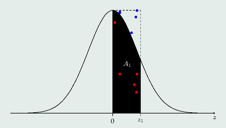
With the use of this function, we gain in precision, especially for large absolute values of the upper integration limit, and especially we gain in processing time. We can also address the Monte Carlo methods, which are especially useful for integrating complex and multidimensional functions. We will present only a rather rudimentary version of this method. The idea is to determine a rectangle that encloses the function we wish to integrate and to bombard the region with random points \((u_1,\, u_2)\) from the uniform distribution.
We count the number of points under the function and determine the corresponding area, based on the proportionality between this number of points and the total number of simulated points in relation to the area under the function in the region of interest relative to the total area of the rectangle. If we know the maximum of the function \(f_{max}\), we can determine this rectangle completely. Thus, the rectangle of interest is defined by the base (value between \(0\) and \(z_1\) in absolute value, with \(z_1\) provided by the user) and by the height (value of the density at the maximum point). Thus, the area of this rectangle is \(A = |z_1|f_{max}\). In the case of the standard normal, the maximum obtained for \(z=0\) is \(f_{max} = 1/\sqrt{2\pi}\), and the area of the rectangle is \(A=|z_1|/\sqrt{2\pi}\). If the area under the curve we wish to estimate is defined by \(A_1\), we can generate uniform numbers \(u_1\) between \(0\) and \(|z_1|\) and uniform numbers \(u_2\) between \(0\) and \(f_{max}\). For each generated value \(u_1\), we compute the density \(f_1=f(u_1)\). Thus, the ratio between the areas \(A_1/A\) is proportional to the ratio \(n/N\), where \(n\) represents the number of points \((u_1, u_2)\) for which \(u_2\le f_1\) and \(N\) the total number of generated points. Hence, the integral is obtained by \(A_1 = |z_1|\times f_{max}\times n/N\), where \(z_1\) is the value of the standard normal for which we wish to compute the area between \(0\) and \(|z_1|\), in order to obtain the distribution function at the point \(z_1\), that is, to obtain \(\Phi(z_1)\). Thus, if \(z_1\le 0\), then \(\Phi(z_1)=0.5-A_1\), and if \(z_1>0\), then \(\Phi(z_1)= 0.5+ A_1\). See the following illustrative figure:
For the particular case of the standard normal, we implemented the following function:
Another way to obtain an approximation of the integral
\[\begin{align*} \int_0^{abs(z)} \dfrac{1}{\sqrt{2\pi}} e^{-t^2/2} dt = \int_0^{abs(z)} \phi(t) dt \end{align*}\]
by Monte Carlo is to generate \(m\) uniform numbers between \(0\) and \(abs(z)\), say \(z_1\), \(z_2\), \(\ldots\), \(z_m\), and obtain
\[\begin{align*} \int_0^{abs(z)} \phi(t) dt \approx \Delta z \left[\dfrac{1}{m} \sum_{i=1}^m \phi(z_i)\right], \end{align*}\]
where \(\phi(t)=1/\sqrt{2\pi}\times\exp\{-t^2/2\}\) is the standard normal density function evaluated at the point \(t\), and \(\Delta z = abs(z) - 0\). The order of error of this process is given by \(O(m^{-1/2})\). The Python program for obtaining the value of the standard normal distribution function \(\Phi(z)\) using these ideas is presented below. By comparing this Monte Carlo alternative with the first one, we can verify that there was a great decrease in the Monte Carlo error in computing this integral in this new approach. Many variants and improvements in this process can be implemented, but we will not discuss them here.
6.4 Gaussian Quadratures
Gaussian quadratures play a preponderant role in statistics, since the main algorithms for obtaining probabilities and quantiles use such methods implicitly. In this section, we will present, in a rather simplified way and without delving into the more technical mathematical aspects, the main Gaussian quadrature method. Those interested in a more detailed treatment of these aspects can consult numerous specific books. We recommend, for example, reading Quarteroni et al. (2000).
The basis of these quadratures is interpolation based on orthogonal polynomials. Their use goes beyond the topic of numerical quadratures and can also be used to approximate least squares solutions and numerical differentiation. An \(n\)-point Gaussian quadrature is one that provides exact results for the integration of a polynomial of degree equal to or less than \(2n-1\). The domain of the quadratures is, without loss of generality and by convention, assumed to be \([-1, 1]\). The general rule for the \(n\)-point Gaussian quadrature of a function \(f(x)\) on the domain \([-1, 1]\) is given by \[ \int_{-1}^1 f(x) dx \approx \sum_{i=1}^n w_i f(x_i), \tag{6.15}\] where \(x_i\) and \(w_i\) are called the nodes and weights, respectively, of the quadrature.
The nodes are values in the interval \([-1, 1]\), and the weights are positive. We must choose them appropriately so that the result of the integral is accurately approximated by the sum on the right. We often use a weight function \(w(x_i)\), such that the integral (6.15) can be represented by \[ \int_{-1}^1 f(x) dx = \int_{-1}^1 w(x)g(x) dx \approx \sum_{i=1}^n w_i g(x_i), \tag{6.16}\] where \(g(x)\) is such that \(f(x)\) \(=\) \(w(x)g(x)\), and \(w_i\) in this case are alternative weights.
For example, for the specific case of the function \(f(x)\) \(=\) \(e^{2x}\), using weights \(w_1\) \(=\) \(w_2\) \(=\) \(1\) and nodes \(x_1\) \(=\) \(\sqrt{3}/3\) and \(x_2\) \(=\) \(-\sqrt{3}/3\), on the domain from \(-1\) to \(1\), results in \[\begin{align*} \int_{-1}^1 e^{2x}dx \approx f(\sqrt{3}/3) + f(-\sqrt{3}/3)=3.4882. \end{align*}\]
The exact value of the integral is \[\begin{align*} \int_{-1}^1 e^{2x}dx =& \left[\dfrac{e^{2x}}{2}\right]_{-1}^{1}=3.6269. \end{align*}\]
It is surprising that the sum \(f(x_1)\) \(+\) \(f(x_2)\) yields exact values for polynomials of degree up to \(3\), \(2n-1\), since \(n\) \(=\) \(2\). What we must do is find mechanisms to obtain the integration weights and nodes. For an integration interval different from \([-1, 1]\), that is, \([a, b]\), \(b>a\), the following transformation does not alter the integration precision: \[ \begin{array}{rl} \int_{a}^b f(x) dx =& \dfrac{b-a}{2} \int_{-1}^1 f\left(\dfrac{b-a}{2}x + \dfrac{a+b}{2}\right)dx\nonumber\\ \approx & \dfrac{b-a}{2} \sum_{i=1}^n w_i f\left(\dfrac{b-a}{2}x_i + \dfrac{a+b}{2}\right). \end{array} \tag{6.17}\]
It is worth emphasizing that the nodes used in the quadratures are the roots of the orthogonal polynomials of some of the commonly used Gaussian families. Among them, we can mention the Legendre, Laguerre, Hermite, Chebyshev, and Jacobi polynomials. We will describe only the Gauss-Legendre quadrature next.
The quadrature called Gauss-Legendre is used for integration intervals defined by \([-1, 1]\) and can be extended to more general intervals if we use expression (6.17). Thus, for the domain \([-1, 1]\), the Gauss-Legendre quadrature can be applied by \[ \int_{a}^b f(x) dx \approx \left\{ \begin{array}{ll} \displaystyle \sum_{i=1}^n w_i f(x_i) & \textrm{for } a=-1\textrm{ and } b=1 \\ \displaystyle \sum_{i=1}^n w_i g(y_i) & \textrm{for } a \textrm{ and } b \textrm{ any reals,} \end{array} \right. \tag{6.18}\] where \(g(y)\) is given by \[ g(y)= \dfrac{b-a}{2} f\left(\dfrac{b-a}{2}x + \dfrac{a+b}{2}\right), \tag{6.19}\] where \(y\) \(=\) \((b-a)x/2\) \(+\) \((b+a)/2\).
The next step, in applying Gaussian quadratures, is to compute the nodes and weights for each of them. We will present this as a sequence of steps. We will use the following quantities for all methods. The scalar \(\mu_0\), defined by
\[\begin{align*} \mu_0=& \int_a^b w(x) dx \end{align*}\]
and the coefficient vectors \(\mathbf{a}\) \((n\) \(\times\) \(1)\) and \(\mathbf{b}\) \((n-1\) \(\times\) \(1)\), where \(n\) is the number of points of the quadrature to be performed.
Subsequently, we will also use a matrix denoted by \(\mathbf{J}\), \((n\) \(\times\) \(n)\), for which we will obtain the eigenvalues and eigenvectors. Since we will use an algebra problem solved by obtaining eigenvalues and eigenvectors, this method is known as the Golub–Welsch algorithm. We will initially describe how to obtain the vectors \(\mathbf{a}\) and \(\mathbf{b}\) and the constant \(\mu_0\) for the Gauss-Legendre quadrature method. Technical details of how this can be done and the theoretical foundations can be found in Quarteroni et al. (2000).
For the Gauss-Legendre quadrature we have:
set \(\mu_0\) \(=\) \(2\);
\(\mathbf{a}=\mathbf{0}\) \((n\) \(\times\) \(1)\);
\(\mathbf{b}=[b_j]\) \((n-1\) \(\times\) \(1)\), such that
\[\begin{align*} b_j =& \dfrac{j}{\sqrt{4j^2 - 1}}, \qquad j=1,\, 2,\, \ldots,\, n-1. \end{align*}\]
Once the necessary quantities \(\mathbf{a}\), \(\mathbf{b}\), and \(\mu_0\) are defined, we must apply the second part of the algorithm to obtain the nodes \(x_i\)’s and the weights \(w_i\)’s, \(i=1\), \(2\), \(\ldots\), \(n\). For this, we use the Golub–Welsch algorithm, by which we determine the matrix \(\mathbf{J}\) from these quantities and determine its eigenvalues and eigenvectors. The matrix \(\mathbf{J}\) is a symmetric tridiagonal matrix defined by \[\begin{align*} \mathbf{J} =& \left[\begin{array}{llllll} a_1 & b_1 & 0 & \ldots & \ldots & \ldots \\ b_1 & a_2 & b_2 & 0 & \ldots & \ldots \\ 0 & b_2 & a_3 & b_3 & 0 & \ldots \\ 0 & \ldots & \ldots & \ldots & \ldots & 0 \\ \ldots & \ldots & 0 & b_{n-2} & a_{n-1} & b_{n-1} \\ \ldots & \ldots & \ldots & 0 & b_{n-1} & a_{n} \end{array} \right]. \end{align*}\]
We determine the eigenvalues and eigenvectors of \(\mathbf{J}\) and denote them by \[\begin{align*} \mathbf{x}^*=& \left[\begin{array}{c} x_1^* \\ x_2^* \\ \vdots\\ x_n^* \end{array} \right] &\textrm{ and }&& \mathbf{P}=& \left[\begin{array}{cccc} p_{11} & p_{21} & \cdots & p_{n1} \\ p_{12} & p_{22} & \cdots & p_{n2} \\ \vdots & \vdots & \ddots & \vdots \\ p_{1n} & p_{2n} & \cdots & p_{nn} \end{array} \right], \end{align*}\]
respectively.
We modify the usual notation for representing the elements of a matrix. Thus, we verify that in matrix \(\mathbf{P}\), the first index of the element \(p_{ij}\) refers to the index of the \(i\)-th eigenvector, and the second index refers to the \(j\)-th element of that eigenvector. This is why the unusual index notation in this matrix. Therefore, each column of \(\mathbf{P}\) corresponds to one of the \(n\) eigenvectors associated with each of the eigenvalues \(x^*_i\) sorted in decreasing order.
Next, we can obtain the nodes (points) by simply taking the eigenvalues in increasing order, that is, the vector of nodes \(\mathbf{x}\), with components \(x_i\), is defined by
\[ \mathbf{x}= \left[\begin{array}{c} x_1 \\ x_2 \\ \vdots\\ x_n \end{array} \right]=\left[\begin{array}{c} x_n^* \\ x_{n-1}^* \\ \vdots\\ x_1^* \end{array} \right], \tag{6.20}\] where \(x_i^*\) is the \(i\)-th eigenvalue of the tridiagonal matrix \(\mathbf{J}\).
We can verify that the nodes are the eigenvalues of this matrix presented in reverse order, that is, in increasing order rather than the usual way of presenting them, which is in decreasing order. Finally, we can obtain the weights as a function of \(\mu_0\) and the first elements of each eigenvector of \(\mathbf{J}\), also considered in reverse order, considering the classical ordering from largest to smallest eigenvalue. This function seeks to perform an appropriate normalization to ensure the validity of the quadrature.
Thus, we have that the quadrature weights are obtained by \[ \mathbf{w}= \left[\begin{array}{l} w_1 \\ w_2 \\ w_3 \\ \vdots \\ w_{n-1} \\ w_n \end{array} \right]=\mu_0\left[\begin{array}{l} p_{n,1}^2 \\ p_{n-1,1}^2 \\ p_{n-2,1}^2 \\ \vdots \\ p_{2,1}^2 \\ p_{1,1}^2 \end{array} \right], \tag{6.21}\] where \(p_{ij}\) is the \(j\)-th element of the \(i\)-th eigenvector of \(\mathbf{J}\) corresponding to the \(i\)-th eigenvalue \(x_i^*\).
We can observe that the values \(w_i\)’s depend on \(p_{ij}\) in reverse order of importance, this order being determined by the eigenvalues of \(\mathbf{J}\).
With the weights, nodes, and weight functions, when the latter is not unity, we can apply the quadrature methods presented earlier. Our next step is to implement functions to obtain the weights and nodes and to provide an example.
In the previous example, we used the sp.linalg.eigh() function from scipy.linalg, since the np.linalg.eig() function does not necessarily return the eigenvalues in order. The eigh function, in turn, returns the eigenvalues sorted, but in increasing order rather than decreasing order, as is done in many other programs. We can apply the quadratures to the normal to illustrate the cases where the limits are not \(-1\) and \(1\), including the previous examples.
In the previous quadratures, we can replace our function that computes the nodes and weights with another one that uses a more efficient method for obtaining eigenvalues and eigenvectors. This method is applicable to symmetric tridiagonal matrices. The following script presents this implementation. We only need to provide a vector with the diagonal of the matrix and another with the elements of the two secondary diagonals, which are identical. The function used was sp.linalg.eigh_tridiagonal() from the scipy library.
6.5 Newton-Raphson
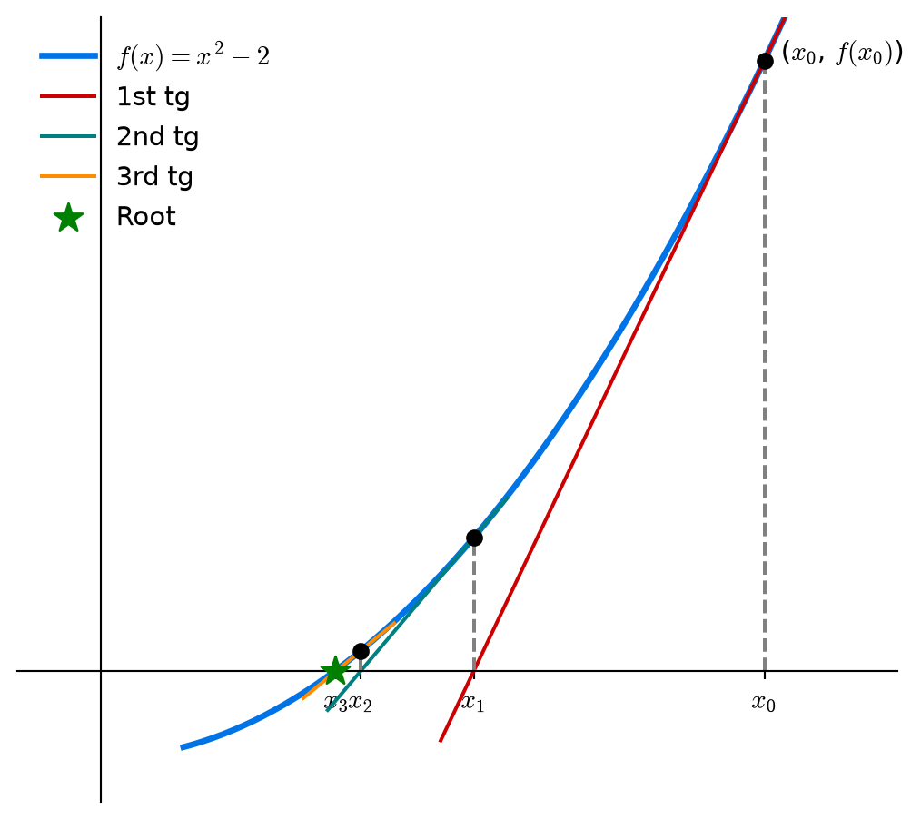
The Newton-Raphson method is used to obtain the solution of a linear or non-linear equation given by \(f(x)=0\). From an initial value \(x_0\), we can draw a tangent line at the point \((x_0, f(x_0))\). The slope of this line is given by the derivative of \(f\) evaluated at \(x_0\). Let \(m\) \(=\) \(f'(x_0)\) be the slope of the tangent line at the point \((x_0, f(x_0))\).
Thus, \[\begin{aligned} m=& \dfrac{\Delta y}{\Delta x}\\ \Delta y =& m \Delta x\\ y-y_0=& f'(x_0)(x-x_0)\\ y=& y_0 + f'(x_0)(x-x_0). \end{aligned}\]
Hence, \[\begin{aligned} f(x)=& f(x_0) + f'(x_0)(x-x_0). \end{aligned}\]
Solving the equation for \(f(x)=0\), we have: \[\begin{aligned} f(x)=& 0\\ f(x_0) + f'(x_0)(x-x_0)=0\\ x= x_0 - \dfrac{f(x_0)}{f'(x_0)} \end{aligned}\]
For any point \(x_n\) of the \(n\)-th repetition of this process, we have \[\begin{aligned} x_{n+1}= x_n - \dfrac{f(x_n)}{f´(x_n)}, \end{aligned}\] which is the expression for solving a linear or non-linear equation by Newton-Raphson. In Figure 6.1 we present an example in which we perform three iterations to illustrate, in search of the solution of the presented equation.
In our particular case, we will present the Newton-Raphson numerical method to obtain the solution of the equation: \[\begin{align*} z =& \Phi^{-1}(p), \end{align*}\] where \(0<p<1\) is the value of the standard normal distribution function, \(\Phi^{-1}(p)\) is the inverse of the standard normal distribution function at the point \(p\), and \(z\) is the corresponding quantile we wish to find given a value of \(p\). We can present this problem by means of the following equation \[\begin{align*} \Phi(z) - p =&0, \end{align*}\] where \(\Phi(z)\) is the standard normal distribution function evaluated at \(z\).
Thus, our objective is to find the zeros of the function \(f(z) = \Phi(z) - p\). In general, we can solve this equation numerically using the Newton-Raphson method, which is an iterative process. Thus, we must have an initial value for the quantile to start the process, and at the \((n+1)\)-th step of the iterative process we can update the value of the quantile by
\[ z_{n+1}= z_n - \dfrac{f(z_n)}{f'(z_n)}, \tag{6.22}\] where \(f'(z_n)\) is the first-order derivative of the function for which we wish to obtain the roots, evaluated at the point \(z_n\). For this particular case, we have that
\[
z_{n+1}= z_n - \dfrac{\left[\Phi(z_n) - p\right]}{\phi(z_n)},
\tag{6.23}\] where \(\phi(z_n)\) is the standard normal density function. As initial values, we will use a rough approximation, since our objective is only to demonstrate the method. Thus, if \(p\) is less than \(0.5\), we will use \(z_0=-0.1\); if \(p>0.5\), we will use \(z_0=0.1\). Obviously, if \(p=0\), the function should return \(z=0\). The function below returns the normal quantiles, given the values of \(p\) between \(0\) and \(1\), the real mean \(\mu\), and the positive real variance \(\sigma^2\), using the Newton-Raphson method and the Hasting phnorm function to obtain the value of the standard normal distribution function.
We could also have used the secant method, since it does not require the first-order derivative but needs two initial values to start the process and has slower convergence. The reader is encouraged to consult Press et al. (1992) for more details. The pnorm function, which uses the trapezoidal method, could also have been used. In that case, the precision would be higher, but the processing time would also be higher. To do this, it would suffice to use the pnorm function as the value of the func argument in the call. It would also be possible to call mcpnorm or pmcnorm or any other efficient implementation we have for the quadrature.
Fortunately, Python also has pre-programmed routines for this and many other probabilistic models, which relieves us of the need to program routines to obtain the distribution functions and inverse distribution functions of the most varied existing probabilistic models.
6.6 Pre-Existing Functions in Python
In Table Table 3.1 we present a good portion of the routines for generating data from the most varied probabilistic models covered by Python. Shortly after the mentioned table, we present the Python procedures from the scipy.stats library to obtain the probability or density function, the distribution function, and the quantile function. We should consult the resources of this library to learn about the most different methods associated with each of its objects.
6.7 Exercises
Compare the precision of the three algorithms for obtaining the normal distribution function presented in this chapter:
pnorm, which uses the trapezoidal method;phnorm, which uses the Hasting method; andpnormal, based on the Gauss-Legendre Gaussian quadrature. Use thenorm.cdf()function fromSciPy Statsas a reference and compute the absolute and relative errors for a vector of supplied quantiles. percentiles.Use different numbers of simulations in the two Monte Carlo methods presented to integrate the normal distribution function and estimate the maximum relative and absolute Monte Carlo error over \(30\) replications for each size. Use the quantiles \(1.00\), \(1.645\), and \(1.96\) and the
norm.cdf()function fromSciPy Statsas a reference.The Cauchy distribution is a particular case of Student’s \(t\) with \(\nu=1\) degree of freedom. The Cauchy density is given by:
\[\begin{align*} f(x) = \dfrac{1}{\pi(1+x^2)} \end{align*}\]
Use the trapezoidal method presented here to implement the computation of the values of the Cauchy distribution function. We can also obtain the distribution function and its inverse analytically. Obtain such functions and implement them in Python. Use the pre-existing
scipy.statsfunctions to check the results obtained, which are expected to be exact for the analytical resolution of the distribution function and its inverse. For the trapezoidal method, compute the absolute and relative errors for some quantiles.Use the most efficient Monte Carlo method described in this chapter to obtain values of the Cauchy distribution function presented in exercise 3. Use some numerical values to illustrate and compare with functions implemented in Python for this case. What should be the minimum number of Monte Carlo simulations required to have reasonable precision?