Basic Statistics
5.2 Solutions
-
5.2.1 The dendrogram (tree diagram) is:
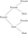
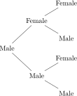
The sample space is obtained by considering all branches of this tree diagram and results in:
\(\seteqnumber{0}{5.}{0}\)\begin{align*} \Omega =&\left \{(FFF),\,(FFM),\,(FMF),\,(FMM),\,(MFF),\,(MFM),\,(MMF),\,(MMM)\right \} \end{align*}
Each point of this space is equally likely, since the probabilities of female and male births are equal and each element of \(\Omega \) has probability \((1/2)^3=1/8\).
-
a) The probability distribution of the random variable \(X\), defined as the number of females, is:
\(x\) \(0\) \(1\) \(2\) \(3\) \(P(X=x)\) \(\dfrac {1}{8}\) \(\dfrac {3}{8}\) \(\dfrac {3}{8}\) \(\dfrac {1}{8}\) For example, the probability \(P(X=1)\) is obtained by the total number of points of \(\Omega \) in which \(X=1\), which in this case is equal to \(3\), relative to the total number of points, which is equal to \(8\).
-
b) The results for the requested events are:
-
i) \(P(X=2)=\dfrac {3}{8}=\)0.3750=37.50%;
-
ii) If \(Y\) represents the number of males, the event \(Y\ge 1\) is equivalent to \(X\le 2\), since if there is \(1\) male in the litter, this implies two females; if there are \(2\) males, it implies \(1\) female; and if there are \(3\) males, it implies \(0\) female. Thus, the probability of the event is:
\(P(Y\ge 1)=P(X\le 2)=P(X=2)+P(X=1)+P(X=0)=\dfrac {3}{8}+\dfrac {3}{8}+\dfrac {1}{8}\) \(=\dfrac {7}{8}=\)0.8750=87.50%;
-
iii) \(P(X\ge 2)=P(X=2)+P(X=3)=\dfrac {3}{8}+\dfrac {1}{8}=\) \(\dfrac {1}{2}=\)0.50=50%;
-
iv) \(P(X\le 1)=P(X=1)+P(X=0)=\dfrac {3}{8}+\dfrac {1}{8}=\) \(\dfrac {1}{2}=\)0.50=50%.
-
-
c) The expected number \(EN\) of litters of \(3\) kittens with exactly \(1\) female is given by the product of the probability of the event \(P(X=1)\) and the total number of litters, that is, \(EN=(3/8)\times 500 \approx 188\) litters. Thus, of the \(500\) we expect \(188\) to have exactly \(1\) female.
-
-
5.2.2 In this case we assume that \(X\), defined as the number of females, has a binomial distribution with parameters \(n=4\) and \(p=5/8\). The probability of success is not \(1/2\), according to Mendel’s laws, since there is a genetic disorder in the breed. We usually use the following notation to say the same thing we just explained: \(X \sim \textrm { Binomial}(n=4,p=5/8)\).
-
a) To obtain the probability distribution of \(X\), we can use the binomial model given by:
\(\seteqnumber{0}{5.}{0}\)\begin{align*} P(X=x)=&\binom {n}{x} p^x(1-p)^{n-x} \end{align*} for \(x=0\), \(1\), \(\ldots \), \(4\).
For example, for the probability \(P(X=0)\) we have:
\(\seteqnumber{0}{5.}{0}\)\begin{align*} P(X=x)=&\binom {4}{0} \left (\dfrac {5}{8}\right )^0\left (1-\dfrac {5}{8}\right )^{4-0}=1\times 1\times \left (\dfrac {3}{8}\right )^4=0.0198. \end{align*}
Thus, we have the following probability distribution:
\(x\) \(0\) \(1\) \(2\) \(3\) \(4\) \(P(X=x)\) 0.0198 0.1318 0.3296 0.3662 0.1526 -
b) The mean is: \(\mu _X= np = 4\times 5/8=\)2.5; and the variance is: \(\sigma ^2_X=np(1-p)=4\times (5/8)\times (3/8)=\)0.9375.
-
c) The expected number \(EN\) of litters is given by the product of the probability of the event of interest \(P(X=x)\) and the total number of litters. For example, for \(X=0\), we have \(P(X=0)\times 1,000=\)0.0198\(\times 1,000=\)19.8\(\approx \)20 litters with no females. The remaining values (rounded) are presented in the following table:
\(x\) \(0\) \(1\) \(2\) \(3\) \(4\) \(P(X=x)\) 0.0198 0.1318 0.3296 0.3662 0.1526 \(EN\) 20 132 330 366 153
-
-
5.2.3 Answer for each of the questions:
-
a) The adequate probabilistic model is the Poisson model, especially if we can assume that the distribution of the bacteria over the slide is random. Thus, \(X \sim \) Poisson\((\lambda =4)\).
-
b) EN\(=P(X\le 1)\times 600\). To obtain the probability of the event of interest we must use the Poisson model given by:
\(\seteqnumber{0}{5.}{0}\)\begin{align*} P(X=x)=& \dfrac {e^{-\lambda }\lambda ^x}{x!}, \end{align*} for \(x=0\), \(1\), \(2\), \(\ldots \) and \(\lambda =4\).
Thus, \(P(X\le 1)=P(X=1)+P(X=0)\), where
\(\seteqnumber{0}{5.}{0}\)\begin{align*} P(X=0)=& \dfrac {e^{-4}\times 4^0}{0!}= 0.0183 &\textrm { and }&& P(X=1)=& \dfrac {e^{-4}\times 4^1}{1!}= 0.0733. \end{align*}
Therefore,
\(\seteqnumber{0}{5.}{0}\)\begin{align*} P(X\le 1)=& P(X=0)+ P(X=1)=0.0183+0.0733=0.0916=9.16\% \end{align*} and the expected number of squares with at most \(1\) bacterium is EN\(=P(X\le 1)\times 600=\) 0.0916\(\times 600\approx 55\).
-
c) \(P(X>2)=P(X=3)+P(X=4)+\ldots \). Since this sum has an infinite number of terms and knowing that the sum of all probabilities is equal to \(1\), then
\(\seteqnumber{0}{5.}{0}\)\begin{align*} P(X>2)=& 1-\left [P(X=0)+P(X=1)+P(X=2)\right ]=1-\left (0.0183+0.0733+\dfrac {e^{-4}\times 4^2}{2!}\right )\\ =& 1-(0.0183+0.0733+0.1465)= 1-0.2381=0.7619=76.19\%. \end{align*}
-
d) \(P(X=0)=\)1.83%.
-
-
5.2.4 The occurrence of diseases per year can be modeled, if random, by the Poisson model. Thus, \(X\sim \) Poisson\((\hat {\lambda }=\bar {X})\).
-
a) The mean is
\(\seteqnumber{0}{5.}{0}\)\begin{align*} \bar {X}=& \dfrac {0\times 55+1\times 40+ \cdots + 5\times 1}{120}=\dfrac {102}{120}=0.85\textrm { diseases/year}. \end{align*}
-
b) The parameter \(\lambda \) can be estimated by \(\hat {\lambda }=\bar {X}=\)0.85. Thus, we can estimate the probability distribution using the Poisson model by:
\(\seteqnumber{0}{5.}{0}\)\begin{align*} P(X=x)=& \dfrac {e^{-0.85}\times 0.85^x}{x!}. \end{align*}
For \(X=0\) and \(X=1\), for illustration purposes, we have:
\(\seteqnumber{0}{5.}{0}\)\begin{align*} P(X=0)=& \dfrac {e^{-0.85}\times 0.85^0}{0!}=0.4274 &&& P(X=1)=& \dfrac {e^{-0.85}\times 0.85^1}{1!}=0.3633. \end{align*}
These and the remaining probabilities are presented in the following table:
\(x\) \(0\) \(1\) \(2\) \(3\) \(4\) \(5\) \(6\) or more \(P(X=x)\) 0.4274 0.3633 0.1544 0.0437 0.0093 0.0016 0.0003 -
c) The expected frequency is given by the product of the probabilities by 120. Thus,
\(x\) \(0\) \(1\) \(2\) \(3\) \(4\) \(5\) \(6\) or more \(P(X=x)\) 0.4274 0.3633 0.1544 0.0437 0.0093 0.0016 0.0003 \(EF\) 51.29 43.60 18.53 5.24 1.12 0.19 0.04 -
d) Since the observed and expected frequencies are relatively close, we can consider that the Poisson model is adequate to model the occurrence of the disease in the studied region.
-
-
5.2.5 Discrete uniform distribution between \(21\) and \(30\).
-
a) Since the support of the variable \(X\), sample size, is \(S_X\) \(=\) \(\{21,\,22,\,\cdots ,30\}\), we have
\(\seteqnumber{0}{5.}{0}\)\begin{align*} P(X=x) =& \dfrac {1}{10}, \textrm { for } x\in S_X, \end{align*} and \(P(X=x)=0\), for other values of \(x\).
-
b) If the cost of each plant is R$ 1.50, considering \(k=10\) \(=\) \(|\Omega |\), and since the mean of the uniform is
\(\seteqnumber{0}{5.}{0}\)\begin{align*} E(X)=&\mu _X = \dfrac {1}{k}\sum _{i=1}^k x_i=\dfrac {1}{10}(21+22+\cdots +30)\\ =& 25.5, \end{align*} then the average weekly cost is 1.50\(\times \) 25.5 \(=\) 38.25 monetary units. If we denote the cost by \(Y\) and verify that the cost is a function of \(X\), given by \(Y\) \(=\) 1.50\(X\), then \(E(Y)\) \(=\) 1.5\(E(X)\). Hence we obtained the previous result.
-
c) The variance of \(X\) is
\(\seteqnumber{0}{5.}{0}\)\begin{align*} V(X) =& \sigma _X^2=\dfrac {1}{k}\left [ \sum _{i=1}^k x_i^2-\dfrac {\left (\displaystyle \sum _{i=1}^k x_i\right )^2}{k}\right ]\\ =& \dfrac {1}{10}\left (6585-\dfrac {255^2}{10}\right )\\ =& 8.25. \end{align*} Since the cost can be interpreted by a transformation of \(X\), given by \(Y\) \(=\) 1.54\(X\). We have that the variance of the cost \(Y\) is \(V(Y)\) \(=\) 1.5\(^2V(X)\) \(=\) 18.5625.
-
d) From Chebyshev’s theorem we have
\(\seteqnumber{0}{5.}{0}\)\begin{align*} P(\mu -k\sigma <X_i<\mu +k\sigma ) \ge 1-\dfrac {1}{k^2}, \quad k>1. \end{align*} Since \(X_i\) must be replaced by the random variable \(Y\) (cost), then we have:
\(\seteqnumber{0}{5.}{0}\)\begin{align*} P(\mu _Y-k\sigma _Y < Y < \mu _Y+k\sigma _Y) \ge 1-\dfrac {1}{k^2}, \quad k>1. \end{align*} Thus, we must find \(k\) such that \(1-1/k^2\ge \)0.95, which results in \(k\ge \) 4.4721. The desired interval is therefore:
\(\seteqnumber{0}{5.}{0}\)\begin{align*} CI_{0.95}(\mu ): & [38.25-4.4721\times \sqrt {18.5625},\,\,38.25+4.4721\times \sqrt {18.5625}]\\ & [18.9823,\,\,\,57.5177]. \end{align*} Thus, at least \(95\%\) of the weeks will have costs between 18.98 and 57.52 monetary units.
-
e) The distribution function is given by
\(\seteqnumber{0}{5.}{0}\)\begin{align*} F(x)=&\sum _{x_i\le x}\dfrac {1}{k}, \forall x\in \mathbb {R} x_i\in S_X. \end{align*} Thus, we have
\(x\) 21 22 23 24 25 26 27 28 29 30 \(F(x)\) 0.10 0.20 0.30 0.40 0.50 0.60 0.70 0.80 0.90 1.00
-
-
5.2.6 Since \(X\) is binomial, then \(\mu _X\) \(=\) \(np\) and \(\sigma ^2_X\) \(=\) \(np(1-p)\). Thus:
-
a) With \(n=30\) and \(p=\)0.1 we have \(\mu _X\) \(=\) \(3\) and \(\sigma ^2_X\) \(=\) 2.70. Thus, for \(k=1\) we have
\(\seteqnumber{0}{5.}{0}\)\begin{align*} P(X<3-\sqrt {2.7})=& P(X<1.36)= P(X=0)+P(X=1)\\ =& \binom {30}{0} \times 0.1^0 \times 0.9^{30} + \binom {30}{1} \times 0.1^1 \times 0.9^{29}\\ =& 0.0424 + 0.1413=0.1837. \end{align*} For \(k=2\) we have,
\(\seteqnumber{0}{5.}{0}\)\begin{align*} P(X<3-2\times \sqrt {2.7})=& P(X<-0.28)= 0. \end{align*}
-
b) With \(n=30\) and \(p=\)0.5 we have \(\mu _X\) \(=\) \(15\) and \(\sigma ^2_X\) \(=\) 7.5. Thus, for \(k=1\) we have
\(\seteqnumber{0}{5.}{0}\)\begin{align*} P(X<15-\sqrt {7.5})=& P(X<12.26)= P(X=0)+P(X=1)+\cdots +P(X=12)\\ =& \binom {30}{0} \times 0.5^0 \times 0.5^{30} + \binom {30}{1} \times 0.5^1 \times 0.5^{29}+\cdots + \binom {30}{12}\times 0.5^{12} \times 0.5^{18}\\ =& 0.1808. \end{align*} For \(k=2\) we have
\(\seteqnumber{0}{5.}{0}\)\begin{align*} P(X<15-2\times \sqrt {7.5})=& P(X<9.52)\\ =& \binom {30}{0} \times 0.5^0 \times 0.5^{30} + \binom {30}{1} \times 0.5^1 \times 0.5^{29}+\cdots + \binom {30}{9}\times 0.5^{9} \times 0.5^{21}\\ =& 0.0214. \end{align*} For \(k=3\) we have
\(\seteqnumber{0}{5.}{0}\)\begin{align*} P(X<15-3\times \sqrt {7.5})=& P(X<6.78) \\ =& \binom {30}{0} \times 0.5^0 \times 0.5^{30} + \binom {30}{1} \times 0.5^1 \times 0.5^{29}+ \cdots + \binom {30}{6} \times 0.5^{6} \times 0.5^{24}\\ =& 0.0007. \end{align*}
-
c) With \(n=30\) and \(p=\)0.9 we have \(\mu _X\) \(=\) \(27\) and \(\sigma ^2_X\) \(=\) 2.7. Thus, for \(k=1\) we have
\(\seteqnumber{0}{5.}{0}\)\begin{align*} P(X<27-\sqrt {2.7})=& P(X<25.36)= P(X=0)+P(X=1)+\cdots +P(X=25)\\ =& \binom {30}{0} \times 0.9^0 \times 0.1^{30} + \binom {30}{1} \times 0.9^1 \times 0.1^{29}+ \cdots + \binom {30}{25} \times 0.9^{25} \times 0.1^{5}\\ =& 0.1755. \end{align*} For \(k=2\) we have
\(\seteqnumber{0}{5.}{0}\)\begin{align*} P(X<27-2\times \sqrt {2.7})=& P(X<23.71)\\ =& \binom {30}{0} \times 0.9^0 \times 0.1^{30} + \binom {30}{1} \times 0.9^1 \times 0.1^{29}+\cdots +\binom {30}{23}\times 0.9^{23}\times 0.1^{7}\\ =& 0.0258. \end{align*}
-
-
5.2.7 Assuming that the binomial model is appropriate to model this case and that \(X\) is the number of germinated seeds in a lot of \(n=100\) with \(p=\)0.95 (admitted by hypothesis as the real value of the probability of success), then the desired probability is: \(P(X>90)\). Thus, under the hypothesis that \(p=\)0.95, we have
\(\seteqnumber{0}{5.}{0}\)\begin{align*} P(X>90) =& P(X=91)+\cdots +P(X=100)\\ =& \binom {100}{91}\times 0.95^{91}\times 0.05^{9}+\cdots +\binom {100}{100}\times 0.95^{100}\times 0.05^{0}\\ =& 0.9718=97.18\%. \end{align*}
The lot has a probability of 97.18% chance of being bought.
The mean and variance are: \(\mu =np\) \(=\) \(95\) and \(\sigma ^2=np(1-p)=\)4.75. We can express the result of Chebyshev’s theorem by
\(\seteqnumber{0}{5.}{0}\)\begin{align*} P(X>\mu +k\sigma ) >& 1-\dfrac {1}{k^2}. \end{align*} Thus, we have that \(\mu +k\sigma \) \(=\) \(95+\)4.75\(k\) \(=\) \(90\). Hence, we have that the absolute value of \(k\) is 2.29. Thus, we have
\(\seteqnumber{0}{5.}{0}\)\begin{align*} P(X>90) =& 1-\dfrac {1}{2.29^2}=0.8093\\ =& 80.93\%, \end{align*} which is a conservative value, as expected by the result of the theorem itself.
-
5.2.8 The probability function of the hypergeometric in this case, with \(n_1=30\) and \(n_2=32\), is:
\(\seteqnumber{0}{5.}{0}\)\begin{align*} P(X=x) =& \dfrac {\dbinom {n_1}{x}\dbinom {N-n_1}{n_2-x}}{\dbinom {N}{n_2}}= \dfrac {\dbinom {30}{x}\dbinom {N-30}{30}}{\dbinom {N}{32}}, \end{align*} for \(\max (0, n_2 - N + n_1) \le x\le \min (n_1, n_2)\), which is equivalent to \(\max (0, 62 - N) \le x\le \min (30, 32)\), which further results in \(\max (0, 62 - N) \le x\le 30\). In the specific experiment, we observed \(x=2\). Thus, the model becomes
\(\seteqnumber{0}{5.}{0}\)\begin{align*} P(X=2) =& \dfrac {\dbinom {30}{2}\dbinom {N-30}{30}}{\dbinom {N}{32}}. \end{align*} We must maximize this probability with respect to \(N\). One way is to do this using a spreadsheet, considering various values of \(N\).
We made a function in \(R\) and observed graphically that the maximum occurs when \(N=479\). The following graph shows this, highlighting the maximum point. The \(R\) program we used is presented right after the graph, having been adapted from the internet.
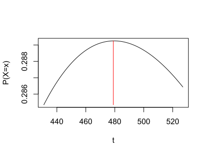
Program: adapted from http://www.sci.csueastbay.edu/~btrumbo/Stat3401/Assign3401/A24.pdf
r <- 30 # red balls in urn
k <- 32 # balls drawn
x <- 2    # red balls drawn
cand <- ceiling(r*k/x) - 1
t <- seq(round(.9*cand), round(1.1*cand))
px <- dhyper(x, r, t-r, k)
mle <- t[px==max(px)]
plot(t, px, type="l",ylab = "P(X=x)")
lines(c(mle,mle),c(max(px),min(px)),col=2)
mle    # MLE as verified by program
cand # MLE from theory
The second alternative is direct through the maximum of the geometric probability function with respect to \(N\). The value of \(n_1n_2/x\) \(=\) \(30\times 32/2\) \(=\) \(480\). Thus, the maximum can be given by either \(480\) or \(479\). Thus, if we calculate the probabilities for these two values, we will see that it is maximized when \(N=479\). This program itself has an error, since it considers only one possibility of maximum with integer value of the initial solution \(n_1n_2/x\). An example in which it fails is with \(n_1=28\), \(n_2=32\), and \(x=2\). In this case the maximum is \(476\) and the program’s solution is \(475\), object cand.
-
5.2.9 If we consider that the distribution of the fungus spore occurs randomly, it is reasonable to adopt the Poisson model to calculate the probability. Thus, if the average per cm\({}^3\) is 0.05, then in \(100\) cm\({}^3\), we will have an average of \(5\) spores. Therefore, if \(X\) refers to the number of spores per \(100\) cm\({}^3\) of soil, then \(X\) \(\sim \) Poi\((\lambda =5)\). The requested probabilities are:
-
a) \(P(X=0)\) \(=\) \(e^{-5}\times 5^0/0!\) \(=\) \(0.0067\).
-
b) \(P(X\ge 3)\) \(=\) \(1\) \(-\) \((P(X=0)+P(X=1)+P(X=2))\) \(=\) \(1\) \(-\) \((0.0067+0.0337+0.0842)\) \(=\) \(1\) \(-\) \(0.1247\) \(=\) \(0.8753\).
-
-
5.2.10 The distribution of the number of failures \(X\) (birth of males) until the occurrence of the first success (birth of a female) in an artificial insemination program is the geometric whose probability function is
\(\seteqnumber{0}{5.}{0}\)\begin{align*} P(X=x) =& (1-p)^x p, \end{align*} for \(x=0\), \(1\), \(2\), \(\cdots \), with \(p=\)0.5. The number of inseminations is therefore \(Y\) \(=\) \(X+1\).
-
a) To guarantee at least \(95\%\) chance of obtaining one success, the birth of \(x\) males is necessary before the occurrence of the first female, according to the following probabilistic statement:
\(\seteqnumber{0}{5.}{0}\)\begin{align*} P(X\le x)=&P(X\le y-1)=\sum _{t=1}^{y}(1-p)^{t-1} p \\ =& \sum _{t=1}^{y} 0.5^{t-1}0.5=\sum _{t=1}^{y} 0.5^t \ge 0.95. \end{align*} The sum on the right refers to the sum of a geometric progression with ratio \(r=1-p=\)0.5 and first term equal to \(p=\)0.5. Thus, this sum is equal to
\(\seteqnumber{0}{5.}{0}\)\begin{align*} 2\left (\dfrac {1}{2}-\dfrac {1}{2^{y+1}}\right )=&1-\dfrac {1}{2^{y}}. \end{align*}
Thus,
\(\seteqnumber{0}{5.}{0}\)\begin{align*} 1-\dfrac {1}{2^{y}} \ge & 0.95, \end{align*} whose solution is
\(\seteqnumber{0}{5.}{0}\)\begin{align*} y \ge & -\dfrac {\ln (0.05)}{\ln (2)}=4.32. \end{align*} Therefore, at least \(5\) inseminations are necessary to guarantee the first success (birth of a female) with at least \(95\%\) probability. If we consider this same problem but with a general value of \(p\) \(\in \) \((0,\,1)\), the ratio of the sum is \(r=1-p\) and the first term is \(p\). Let us consider that the \(95\%\) value is replaced by a minimum probability \(\gamma \), to make the problem general. Thus,
\(\seteqnumber{0}{5.}{0}\)\begin{align*} P(X\le x)=&P(X\le y-1)=\sum _{t=1}^{y}(1-p)^{t-1} p \ge \gamma . \end{align*} If we further denote the sum of the cumulative probabilities up to \(y\) by \(S_y\), we will have \(S_y\) \(=\) \(1-(1-p)^y\). Thus, the general solution is
\(\seteqnumber{0}{5.}{0}\)\begin{align*} y \ge & \dfrac {\ln (1-\gamma )}{\ln (1-p)}. \end{align*}
-
b) Waiting “until” the third attempt to have the first success means that the desired probability implies having \(2\) failures before the first female is born on the third attempt (insemination) or \(1\) failure on the second attempt or success on the first attempt. This probability is given by
\(\seteqnumber{0}{5.}{0}\)\begin{align*} P(X\le 2) =&\sum _{x=0}^{2} (1-p)^xp\\ =&\left (\dfrac {1}{2}\right )^0\dfrac {1}{2} +\left (\dfrac {1}{2}\right )^1\dfrac {1}{2}+ \left (\dfrac {1}{2}\right )^2\dfrac {1}{2}\\ =&0.5000+0.2500+ 0.1250=87.50\%. \end{align*}
-
-
5.2.11 This case refers to the same previous experiment, but with the waiting for more than one success in repetitions of the Bernoulli trials (inseminations). Thus, we have that the adequate model is the negative binomial. The probability function with \(r\) successes and probability of success \(p\) of the variable \(X\) referring to the number of failures until the \(r\)-th success is:
\(\seteqnumber{0}{5.}{0}\)\begin{align*} P(X=x|r) = \dbinom {x+r-1}{x}p^r(1-p)^x, \end{align*} for \(x = 0\), \(1\), \(2\), \(3\), \(\cdots \). We also have that \(p=\)0.5 is the probability of being born female in an insemination.
-
a) To have the second success in the third insemination, it indicates that we had \(1\) failure before this last success occurred. Thus, the desired probability
\(\seteqnumber{0}{5.}{0}\)\begin{align*} P(X=1|r=2) =& \dbinom {1+2-1}{1}0.5^2(1-0.5)^1=0.25=25\%. \end{align*}
-
b) This case is a little more complex than the geometric case, since in our sum of the terms of the cumulative probabilities, we will not have a geometric progression as in that case. Thus, the alternative is to compute the cumulative probabilities until the requested minimum probability value (in this case \(95\%\)) is reached. Therefore, using a program to help we have
\(\seteqnumber{0}{5.}{0}\)\begin{align*} P(\le 0|r=3) =&\dbinom {x+r-1}{x}p^r(1-p)^x\\ =& \dbinom {0+3-1}{0}0.5^3(1-0.5)^0=0.1250, \end{align*} which does not guarantee the minimum of \(95\%\). We advanced to the next value of \(x\) and obtained
\(\seteqnumber{0}{5.}{0}\)\begin{align*} P(\le 1|r=3) =& \dbinom {0+3-1}{0}0.5^3(1-0.5)^0+ \dbinom {1+3-1}{1}0.5^3(1-0.5)^1\\ =& 0.1250+0.1875=0.3125, \end{align*} which again does not guarantee the minimum of \(95\%\). If we proceed with this method we will see that \(P(X\le 7|r=3)=\)0.9453125 and \(P(X\le 8|r=3)=\)0.9672852. Thus, we need at least \(8\) failures before the third success. Thus, the total number of inseminations necessary is \(r+x\) \(=\) \(3+8\) \(=\) \(11\) inseminations to guarantee with at least \(95\%\) chance that the third success (birth of the third female) occurs.
-
c) The expected value (with \(r=3\)) is
\(\seteqnumber{0}{5.}{0}\)\begin{align*} \mu _X =& \dfrac {r(1-p)}{p} = \dfrac {3\times (1-0.5)}{0.5}=3. \end{align*} Thus, we need on average \(3\) failures to reach the three successes. Thus, the average number of inseminations necessary is equal to \(6\).
-
-
5.2.12 In this case, we have the distribution of a binomial variable conditioned on the conditions \(X\ge 1\) and \(X\ge 2\). Thus, for the first case
\(\seteqnumber{0}{5.}{0}\)\begin{align*} P(X=x|X\ge 1) =& \dfrac {P(\{X=x\}\cap \{X\ge 1\})}{P(X\ge 1)}\\ =& \dfrac {P(X=x)}{1-P(X=0)}, \quad x=1,2,\cdots ,n. \end{align*} Thus, considering a binomial with \(n=8\) and \(p=\)0.5, this probability function becomes
\(\seteqnumber{0}{5.}{0}\)\begin{align*} P(X=x|X\ge 1) =&\dfrac {\binom {8}{x}p^x(1-p(8-x))}{0.9960938}, \quad x=1,2,\cdots ,8. \end{align*} We compute the probabilities in each case and the results are:
\(x\) 1 2 3 4 5 6 7 8 \(p(x)\) 0.0314 0.1098 0.2196 0.2745 0.2196 0.1098 0.0314 0.0039 We can verify that the sum of the values with respect to the new support set results in \(1\).
For the second case, the procedure is similar:
\(\seteqnumber{0}{5.}{0}\)\begin{align*} P(X=x|X\ge 2) =& \dfrac {P(\{X=x\}\cap \{X\ge 2\})}{P(X\ge 2)}\\ =& \dfrac {P(X=x)}{1-P(X\le 1)}, \quad x=2,3,\cdots ,8. \end{align*} Thus, this probability function is
\(\seteqnumber{0}{5.}{0}\)\begin{align*} P(X=x|X\ge 2) =&\dfrac {\binom {8}{x}p^x(1-p(8-x)}{0.9648438}, \quad x=2,3,\cdots ,8. \end{align*} We compute the probabilities in each case and the results are:
\(x\) 2 3 4 5 6 7 8 \(p(x)\) 0.1134 0.2267 0.2834 0.2267 0.1134 0.0324 0.0040 -
5.2.13 The probability function of the beta-binomial distribution with parameters \(\alpha \) and \(\beta \) is given by
\(\seteqnumber{0}{5.}{0}\)\begin{align*} P(X=x) =& \dbinom {n}{x}\dfrac {\Gamma (\alpha +\beta )}{\Gamma (\alpha ) \Gamma (\beta )}\dfrac {\Gamma (x+\alpha )\Gamma (n+ \beta -x)}{\Gamma (n+\alpha +\beta )}, \end{align*} for \(x=0\), \(1\), \(2\), \(\cdots \), \(n\). If we consider \(\alpha \) \(=\) \(\beta \) \(=\) \(1\) we have that \(\Gamma (\alpha +\beta )\) \(=\) \(\Gamma (2)\) \(=\) \(1\), \(\Gamma (\alpha )\) \(=\) \(\Gamma (\beta )\) \(=\) \(1\) and
\(\seteqnumber{0}{5.}{0}\)\begin{align*} \dfrac {\Gamma (x+\alpha )\Gamma (n+ \beta -x)}{\Gamma (n+\alpha +\beta )}=& \dfrac {\Gamma (x+1)\Gamma (n+1-x)}{\Gamma (n+2)}=\dfrac {x!(n-x)!}{(n+1)!}\\ =& \dfrac {x!(n-x)!}{(n+1) n!}=\dfrac {1}{n+1}\dfrac {1}{\binom {n}{x}}. \end{align*} Thus,
\(\seteqnumber{0}{5.}{0}\)\begin{align*} P(X=x) =& \dbinom {n}{x}\dfrac {1}{1}\dfrac {1}{n+1}\dfrac {1}{\binom {n}{x}}\\ =& \dfrac {1}{n+1}, \end{align*} for \(x=0\), \(1\), \(2\), \(\cdots \), \(n\) and represents the probability function of a discrete uniform with \(n+1\) elements in its support, as we wanted to show.
The mean and variance are:
\(\seteqnumber{0}{5.}{0}\)\begin{align*} \mu _{X} =& \dfrac {n\alpha }{\alpha +\beta } & \textrm { and } && \sigma ^2_{X}=& \dfrac {n\alpha \beta (n+\alpha +\beta )}{(\alpha +\beta )^2 (\alpha +\beta +1)}, \end{align*}
\(\seteqnumber{0}{5.}{0}\)\begin{align*} \mu _{X} =& \dfrac {n}{2} & \textrm { and } && \sigma ^2_{X}=& \dfrac {n(n+2)}{12}. \end{align*} The mean and variance of a random variable \(Y\) with discrete uniform distribution with support in \(S_Y\) \(=\) \(\{a\), \(a+1\), \(\cdots \), \(b-1\), \(b\}\) are
\(\seteqnumber{0}{5.}{0}\)\begin{align*} \mu _{X} =& \dfrac {a+b}{2} & \textrm { and } && \sigma ^2_{X}=& \dfrac {(b-a+1)^2-1}{12}. \end{align*} If we set \(a=0\) and \(b=n\), we will have exactly the quantities previously presented, after some algebraic simplifications.
-
5.2.14 Let us demonstrate the mean and variance of the discrete uniform with support \(S_X\) \(=\) \(\{1\), \(2\), \(\cdots \), \(k\}\). The mean
\(\seteqnumber{0}{5.}{0}\)\begin{align*} E(X)=&\mu _X = \dfrac {1}{k}\sum _{i=1}^k x_i=\dfrac {1}{k}(1+2\cdots +k)\\ =& \dfrac {k(k+1)/2}{k} \quad \textrm {(sum of an arithmetic progression)}\\ =& \dfrac {k+1}{2}. \end{align*} The variance is:
\(\seteqnumber{0}{5.}{0}\)\begin{align*} V(X) =& \sigma _X^2=\dfrac {1}{k}\left [\sum _{i=1}^k x_i^2-\dfrac {\left (\displaystyle \sum _{i=1}^k x_i\right )^2}{k}\right ]\\ =& \dfrac {1}{k}\left [\dfrac {k^3}{3}+\dfrac {k^2}{2}+\dfrac {k}{6}- \dfrac {\left (k(k+1)/2\right )^2}{k} \right ]\\ =& \dfrac {1}{k}\left [\dfrac {k^3}{3}+\dfrac {k^2}{2}+\dfrac {k}{6}- \dfrac {k^3}{4}-\dfrac {k^2}{2}-\dfrac {k}{4}\right ]\\ =& \dfrac {k^2}{3}+ \dfrac {k}{2}+\dfrac {1}{6}- \dfrac {k^2}{4}-\dfrac {k}{2}-\dfrac {1}{4}\\ =& \dfrac {k^2-1}{12}, \end{align*} as we wanted to show.
For the second part, let us consider that the values of the provided support result from a transformation of variables. If \(X\) is the original variable with support between \(1\) and \(k\), then \(Y\) \(=\) \(X-1\) is a random variable with support with integer values between \(0\) and \(k-1\). Using the linearity of the expectation, we have
\(\seteqnumber{0}{5.}{0}\)\begin{align*} E(Y) =& E(X-1)=E(X)-1=\dfrac {k+1}{2}-1\\ =& \dfrac {k-1}{2}. \end{align*} For the variance we have:
\(\seteqnumber{0}{5.}{0}\)\begin{align*} V(Y) =& V(X-1)=V(X)=\dfrac {k^2-1}{12}, \end{align*} since the variance does not change when a constant is subtracted from a random variable.