Basic Statistics
10.2 Solutions
-
10.2.1 Let us divide our results into the different tests or graphical procedures. Let us start with the tests.
-
a) Considering the sample of size \(n\) \(=\) \(15\), we have the results presented in the following table for the Shapiro-Wilk test. We applied the estimation formulas for the \(a_i\)’s presented in the Book, choosing those of greater accuracy. We also present the results of the estimates using the extremely accurate methods presented by Royston (1993) and described in detail in Ferreira (2018). We made two functions in R to perform these calculations more easily. The function bSW.test applies the Shapiro-Wilk test with the approximate version, in which most of the expressions were obtained for this Book only. The second function SW.test uses a more accurate version of the test, since it is based on the proposal of Royston (1993).
The two functions for applying the SW test, together with the existing function in R itself, and the data of the example are:
# Function to apply the Shapiro-Wilk's
# normality test - version of my book
bSW.test <- function(x)
{
  n <- length(x)
  pis <- ((1:n) - 0.375) / (n + 0.25)
  mi <- qnorm(pis)
  if (n == 3)
    ai <- c(-2^0.5/2, 0, 2^0.5/2) else
  {
     ais <- 2 * mi[2:(n-1)]
     if (n<=20) a1 <- gamma(n/2)/(2*sqrt(2)*gamma((n+1)/2))+
     gamma((n+1)/2)/(2*sqrt(2)*gamma((n+2)/2)) else
     if (n<=50) a1 <- gamma((n+1)/2)/(sqrt(2)*gamma((n+2)/2)) else
     { # n > 50
           a12 <- mi[1]^2/sum(mi^2)
           a1 <- 30*gamma((n+1)/2)/(sqrt(2)*gamma((n+2)/2))/n+
                      (n-30)/n*a12
     }
     a1s <- a1 / (1-2*a1)*sum(ais^2)
     ais <- c(-(a1s^0.5),ais,(a1s^0.5))
     ai <- ais/(sqrt(sum(ais^2)))
  }
  w <- sum(ai * sort(x))^2 / ((n-1)*var(x))
  if (n == 3)
  {
    valor.p <- 6 / pi * (asin(sqrt(w)) - asin(sqrt(0.75)))
  } else
  {
    if (n <= 11)
    {
      lamb <- -2.273+0.459*n
      U <- log(1-w)
      if (lamb>U) Y <- -log(lamb-U) else Y<- Inf
      muy <- 0.544 - 0.39978*n +
              0.025054*n^2 - 0.0006714*n^3
      sigY <- exp(1.3822 - 0.77857*n +
                   0.062767*n^2- 0.0020322*n^3)
      Zc <- (Y - muy) / sigY
      valor.p <- 1 - pnorm(Zc)
    } else
    {
      u <- log(n)
      Y <- log(1-w)
      muy <- -1.5861 - 0.31082*u -
               0.083751*u^2 + 0.0038915*u^3
      sigY <- exp(-0.4803-0.082676*u+0.0030302*u^2)
      Zc <- (Y - muy) / sigY
      valor.p <- 1 - pnorm(Zc)
    }
  }
  plot(ai,sort(x),xlab="a's",ylab="x's")
  abline(lm(sort(x)~ai),col="red")
  return(list(w=w,p.value=valor.p))
}

# Function to apply the Shapiro-Wilk's
# normality test - version of Royston(1993)
SW.test <- function(x)
{
  n <- length(x)
  if (n == 3)
    a <- c(-sqrt(2)/2,0,sqrt(2)/2) else
  {
    p <- ((1:n) - 0.375) / (n + 0.25)
    m <- qnorm(p)
    sm2 <- sum(m^2)
    c <- m / sqrt(sm2)
    u <- 1 / sqrt(n)
    if (n <= 5)
    {
      an <- c[n]+0.221157*u-0.14798*u^2-
        2.071190*u^3+4.434685*u^4-2.706056*u^5
      phi <- (sm2 - 2 * m[n]^2) / (1 - 2 * an^2)
      a <- c(-an,m[2:(n-1)]/phi^0.5,an)
    } else
    {
      an <- c[n]+0.221157*u-0.14798*u^2-
        2.071190*u^3+4.434685*u^4-2.706056*u^5
      an1 <- c[n-1]+0.042981*u-0.293762*u^2-
        1.752461*u^3+5.682633*u^4-3.582633*u^5
      phi <- (sm2 - 2 * m[n]^2 - 2 * m[n-1]^2) /
              (1 - 2 * an^2 - 2 * an1^2)
      a <- c(-an,-an1,m[3:(n-2)]/phi^0.5,an1,an)
    }
  }
  w <- (sum(a*sort(x)))^2 / ((n - 1) * var(x))
  if (n == 3)
    p.value <- 6/pi*(asin(sqrt(w))-asin(sqrt(0.75))) else
  { # n>3
     if (n <= 11)
     {
       gam <- -2.273+0.459 * n
       Y <- -log(gam - log(1 - w))
       muY <- 0.5440-0.39978*n+
          0.025054*n^2-0.0006714*n^3
       sigY<-exp(1.3822-0.77857*n+
                  0.062767*n^2-0.0020322*n^3)
       Z <- (Y - muY) / sigY
       p.value <- 1 - pnorm(Z)
     } else
     {
       Y <- log(1- w)
       u <- log(n)
       muY <- -1.5861-0.31082*u-
               0.083751*u^2+0.0038915*u^3
       sigY<-exp(-0.4803-0.082676*u+0.0030302*u^2)
       Z <- (Y - muY) / sigY
       p.value <- 1 - pnorm(Z)
     }
  }
  plot(a,sort(x),xlab="a's",ylab="x's")
  abline(lm(sort(x)~a),col="red")
  return(list(w=w,p.value=p.value))
}

# Example: Exercise 10.5.1
x <- c(8.52,9.07,11.90,9.43,4.32,
       5.77,8.52,5.95,5.56,9.02,
       12.08,8.06,9.96,6.02,8.69)
bSW.test(x)
SW.test(x)
shapiro.test(x)#R function for SW's test
The values of the test statistic, using the Book’s version and that of Royston (1993), are
\(\seteqnumber{0}{10.}{0}\)\begin{align*} W=& \dfrac {\left (\displaystyle \sum _{i=1}^n \hat {a}_i X_{(i)}\right )^2}{\displaystyle \sum _{i=1}^{n} X^2_i-\dfrac {\left (\displaystyle \sum _{i=1}^{n} X_i\right )^2}{n}} =\dfrac {8.306^2}{72.99}\\ =& 0.9452 \end{align*} and
\(\seteqnumber{0}{10.}{0}\)\begin{align*} W=& \dfrac {\left (\displaystyle \sum _{i=1}^n \hat {a}_i X_{(i)}\right )^2}{\displaystyle \sum _{i=1}^{n} X^2_i-\dfrac {\left (\displaystyle \sum _{i=1}^{n} X_i\right )^2}{n}} =\dfrac {8.296^2}{72.99}\\ =& 0.9430, \end{align*} respectively.
Once the value of the statistic is obtained, using the Book’s version, we must obtain certain necessary quantities, which for this case, \(n>11\), are
\(\seteqnumber{0}{10.}{0}\)\begin{align*} x =& \ln (n) = \ln (15) = 2.7081\\ Y=& \ln (1-W)=-2.9036. \end{align*} where the mean and standard deviation of \(Y\) are
\(\seteqnumber{0}{10.}{0}\)\begin{align*} \mu _Y=& -2.9647 & \textrm { and }&& \sigma _Y&= 0.5056. \end{align*}
Therefore, the standardized value of \(Y\) is
\(\seteqnumber{0}{10.}{0}\)\begin{align*} Z_c=& \dfrac {Y-\mu _Y}{\sigma _Y}=\dfrac {-2.9036+2.9647}{0.5056}= 0.1210. \end{align*}
Thus,
\(\seteqnumber{0}{10.}{0}\)\begin{align*} \textrm {$p$-value} =& P(Z>0.1210) = 0.4519. \end{align*}
Therefore, the null hypothesis of normality should not be rejected at the nominal significance level of \(5\%\).
For the second option, the more accurate test using the results of Royston (1993), we have that \(Z_c\) \(=\) 0.1975 and the \(p\)-value \(=\) 0.4217. Thus, the conclusion is the same as before. Thus, we can conclude that our approximation is quite reasonable. Of course we performed Monte Carlo simulations to validate and not just a simple example like this, before publishing the Book. We suggest that readers use the more accurate version, either the second function of the program above or the shapiro.test function of the R program, also presented in the program above. The advantage of our function over that of R is that it makes a quantile-quantile type graph, in which one of the quantiles is related to the expectation of the normalized order statistics (quantities \(a_i\)’s) and the other is the observed order statistics. This graph, using the calculation with the expressions of Royston (1993), is presented below:
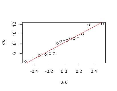
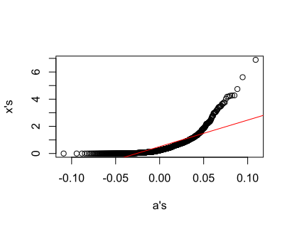
We verify that the least squares line fits the observed points \((\hat {a}_i\), \(x_{(i)})\) reasonably well, indicating the normality of the data. We performed a simulation with \(n\) \(=\) \(1000\) data from a gamma(0.5) distribution and the fitted least squares line completely deviates from the dispersion of the points, indicating, as expected, the non-normality of the data.
-
b) The second case to be considered is the tests of departures from skewness and kurtosis of D’Agostino et al. (1990). After the example, we present again three functions for automatic application of these tests, which are laborious to apply, but not difficult.
The sample mean and standard deviation are \(\bar {X}\) \(=\) 8.1913 days and \(S\) \(=\) 2.2833 t/ha. The estimates of skewness and kurtosis are \(\sqrt {b_1}\) \(=\) 0.041948, \(b_2\) \(=\) 2.2116 and \(g_2\) \(=\) \(-\)0.59356.
-
i) Skewness test
The null and alternative hypotheses for the skewness test are
\(\seteqnumber{0}{10.}{0}\)\begin{align*} H_0: \sqrt {\beta _1}=0 \qquad \qquad \textrm { versus } \qquad \qquad H_1: \sqrt {\beta _1}\ne 0. \end{align*}
-
1) First alternative
The test statistic is
\(\seteqnumber{0}{10.}{0}\)\begin{align*} Z_1=& \sqrt {b_1}\sqrt {\dfrac {(n+1)(n+3)}{6(n-2)}}\\ =& 0.041948 \sqrt {\dfrac {(15+1)(15+3)}{6(15-2)}} =& 0.080605. \end{align*}
Since \(Z_1\) \(\le \) \(Z_{0.025}\) \(=\) 1.96, \(H_0\) is not rejected and it is concluded that the distribution is symmetric. Note: The program will only apply this approximation if \(n<7\), which is not the case.
-
2) Second alternative
This is an improved approximation relative to the first alternative. For this, it is necessary to calculate the following values
\(\seteqnumber{0}{10.}{0}\)\begin{align*} B=& \dfrac {3(n^2+27n-70)(n+1)(n+3)}{(n-2)(n+5)(n+7)(n+9)} \\ =& \dfrac {3(15^2+27\times 15-70)(15+1)(15+3)}{(15-2)(15+5)(15+7)(15+9)} = 3.5245, \\ C=& \sqrt {2(B-1)}-1= \sqrt {2(3.5245-1)}-1=1.2470,\\ D=& \sqrt {C} =\sqrt {1.2470} = 1.1167,\\ E=& \dfrac {1}{\sqrt {\ln (D)}} = \dfrac {1}{\sqrt {\ln (1.1167)}} = 3.0101,\\ F=& \dfrac {Z_1}{\sqrt {2/(C-1)}} = \dfrac {0.080605}{\sqrt {2/(1.1167-1)}} =0.028326. \end{align*}
Thus,
\(\seteqnumber{0}{10.}{0}\)\begin{align*} Z_{1c} =& E \ln \left (F+\sqrt {F^2+1}\right )\\ =& 3.0101\times \ln \left (0.028326+\sqrt {0.028326^2+1}\right )\\ =& 0.0853. \end{align*}
Since the value \(|Z_{1c}|\) \(\le \) 1.96, the conclusion is, therefore, the same as the previous item, that is, there are no skewness departures in the distribution, considering the nominal significance level of \(5\%\). In this second case (as could have been done in the first) we computed the \(p\)-value which was 0.93206. Thus, since the \(p\)-value>0.05, the null hypothesis should not be rejected. This approximation is more adequate and the value of the statistic differs from the previous value, which is 0.0806.
-
-
ii) Hypothesis about kurtosis
The null and alternative hypotheses are
\(\seteqnumber{0}{10.}{0}\)\begin{align*} H_0: {\beta _2}=3 \qquad \qquad \textrm { versus } \qquad \qquad H_1: {\beta _2}\ne 3. \end{align*}
-
1) First alternative
The test statistic is
\(\seteqnumber{0}{10.}{0}\)\begin{align*} Z_2 =& \left (b_2-3+ \dfrac {6}{n+1}\right ) \sqrt {\dfrac {(n+1)^2(n+3)(n+5)}{24 n(n-2)(n-3)}} \\ =& \left (2.2116-3+ \dfrac {6}{15+1}\right ) \sqrt {\dfrac {(15+1)^2(15+3)(15+5)}{24\times 15(15-2)(15-3)}}\\ =& -0.52954. \end{align*}
Since \(|Z_2|\) \(<\) 1.96, then \(H_0\) should not be rejected, that is, the distribution cannot be considered different from mesokurtic, at the nominal significance level of \(5\%\).
-
2) Second alternative
This is an improved option of the test and the gamma estimate of kurtosis is
\(\seteqnumber{0}{10.}{0}\)\begin{align*} g_2 =& \dfrac {(n-1)\left [(n+1)b_2-3(n-1)\right ]}{(n-2)(n-3)} \\ =& \dfrac {(15-1)\left [(15+1)2.2116-3(15-1)\right ]}{(15-2)(15-3)}\\ =& -0.59356. \end{align*}
The other quantities necessary to obtain the best approximation are
\(\seteqnumber{0}{10.}{0}\)\begin{align*} H=& \dfrac {(n-2)(n-3)|g_2|}{(n+1)(n-1)} \sqrt {\dfrac {(n+1)^2(n+3)(n+5)}{24n (n-2)(n-3)}} \\ =& \dfrac {(15-2)(15-3)|-0.59356|}{(15+1)(15-1)} \sqrt {\dfrac {(15+1)^2(15+3)(15+5)}{24\times 15(15-2)(15-3)}}\\ =& 0.52954,\\ J=& \dfrac {6(n^2-5n+2)}{(n+7)(n+9)}\sqrt {\dfrac {6(n+3)(n+5)}{n (n-2)(n-3)}} \\ =& \dfrac {6(15^2-5\times 15+2)}{(15+7)(15+9)} \sqrt {\dfrac {6(15+3)(15+5)}{15 (15-2)(15-3)}}\\ =& 1.6595,\\ K=& 6 +\dfrac {8}{J}\left [\dfrac {2}{J}+\sqrt {1+\dfrac {4}{J^2}}\right ]\\ =& 6 +\dfrac {8}{1.6595} \left [\dfrac {2}{1.6595}+\sqrt {1+\dfrac {4}{1.6595^2}}\right ]\\ =& 19.3591,\\ L=& \dfrac {1-2K^{-1}}{1+H\sqrt {2(K-4)^{-1}}}\\ =& \dfrac {1-2\times 19.3591^{-1}}{1+0.52954 \sqrt {2(19.3591-4)^{-1}}}\\ =& 0.75283. \end{align*}
Therefore, the test statistic is
\(\seteqnumber{0}{10.}{0}\)\begin{align*} Z_{2c} =& \dfrac {1-2(9K)^{-1}-\sqrt [3]{L}}{\sqrt {2(9K)^{-1}}}\\ =& \dfrac {1-2(9\times 19.3591)^{-1}-\sqrt [3]{0.75283}}{\sqrt {2(9 \times 19.3591)^{-1}}}\\ =& 0.7357. \end{align*}
Since \(|Z_{2c}|\) \(<\) 1.96, then \(H_0\) should not be rejected, that is, the distribution cannot be considered different from mesokurtic.
-
-
iii) Joint test of skewness and kurtosis:
The null and alternative hypotheses for the joint skewness and kurtosis test are
\(\seteqnumber{0}{10.}{0}\)\begin{align*} H_0: \sqrt {\beta _1}=0 \textrm { and } \beta _2=3 \textrm { versus } H_1: \sqrt {\beta _1}\ne 0 \textrm { or } \beta _2\ne 3. \end{align*}
The test statistic is
\(\seteqnumber{0}{10.}{0}\)\begin{align*} \chi ^2_c =& 0.08525^2+0.73566^2\\ =& 0.5485. \end{align*} Considering the chi-square distribution with \(\nu =2\) degrees of freedom, we have the following \(p\)-value \(=\) \(P(\chi ^2_{2}\ge \)0.5485) \(=\) 0.7602. Since the value is less than 0.05, we should not reject \(H_0\) of symmetric and mesokurtic distribution. Thus, we have that there is no evidence of normality departures considering the nominal level of \(5\%\). This result, although it is an indirect normality test, since symmetry and mesokurtosis are necessary but not sufficient conditions, agrees with the Shapiro-Wilk test, previously presented. A protocol that we recommend is to apply the joint test. If there is no significance, we end the process and conclude in favor of normality. Otherwise, we apply each test individually (skewness and kurtosis) to identify the departure or departures from normality that occurred.
The R program for these cases is:
# Function to apply the D'Agostino's test # for departure from normality, based on # skewness departure: improved DagSkewNormTest <- function(x) { n <- length(x) srb1 <- (sum((x-mean(x))^3)/n) / ((n-1)*var(x)/n)^1.5 z1 <- srb1 * ((n+1)*(n+3)/(6*(n-2)))^0.5 if (n < 7) z1c <- z1 else { B <- 3*(n^2+27*n-70)*(n+1)*(n+3) / ((n-2)*(n+5)*(n+7)*(n+9)) C <- sqrt(2*(B-1))-1 D <- sqrt(C) E <- 1 / sqrt(log(D)) FF <- z1 / sqrt(2 / (C - 1)) z1c <- E*log(FF +sqrt(FF^2 + 1)) } p.value <- 2 * (1 - pnorm(abs(z1c))) return(list(zc = z1c, p.value = p.value, Skewness=srb1)) } # Function to apply the D'Agostino's test # for departure from normality, based on # kurtosis departure: improved DagKurtNormTest <- function(x) { n <- length(x) b2 <- (sum((x-mean(x))^4)/n) / ((n-1)*var(x)/n)^2 g2 <- (n-1)*((n+1)*b2-3*(n-1))/((n-2)*(n-3)) z2 <- (b2 - 3 + 6 / (n + 1)) * ((n+1)^2*(n+3)*(n+5)/(24*n*(n-2)*(n-3)))^0.5 if (n < 4) z2c <- z2 else { H <- (n-2)*(n-3)*abs(g2)/((n+1)*(n-1)) * ((n+1)^2*(n+3)*(n+5)/(24*n*(n-2)*(n-3)))^0.5 J <- 6*(n^2-5*n+2)/((n+7)*(n+9)) * (6*(n+3)*(n+5)/ (n*(n-2)*(n-3)))^0.5 K <- 6 + 8/J*(2/J+sqrt(1+4/J^2)) L <- (1-2*1/K)/(1+H*sqrt(2/(K-4))) z2c <- (1-2/(9*K)-L^(1/3))/ sqrt(2/(9*K)) } p.value <- 2 * (1 - pnorm(abs(z2c))) return(list(zc = z2c, p.value = p.value, Kurtosis=b2, gKurt=g2)) } # Function to apply the D'Agostino's # omnibus test for Skewness and Kurtosis # departure: indirect normality test OmnibusNormTest <- function(x) { chi2c <- DagSkewNormTest(x)$zc^2 + DagKurtNormTest(x)$zc^2 nu <- 2 p.value <- 1 - pchisq(chi2c, nu) return(list(chi2c = chi2c, p.value = p.value)) } # Example: Exercise 10.5.1 x <- c(8.52,9.07,11.90,9.43,4.32, 5.77,8.52,5.95,5.56,9.02, 12.08,8.06,9.96,6.02,8.69) OminbusNormTest(x) DagSkewNormTest(x) DagKurtNormTest(x) -
-
c) Computing the correlation between the columns \(\hat {m}_i\) and \(X_{(i)}\) of the table of item (i), we have \(r_Q\) \(=\) 0.97477. The critical value, obtained in Table 10.2 (Book), with \(n=15\) and \(\alpha =\)0.05 is 0.9389. Since the calculated value is greater than the tabulated one, there is no reason to reject the null hypothesis of normality.
For the graphical procedures we have the following results:
\(j\) \(P_j\) \(\hat {m}_j\) \(\hat {P}_j\) \(x_{(j)}\) 1 0.0410 -1.7394 0.0396 4.32 2 0.1066 -1.2450 0.1165 5.56 3 0.1721 -0.9458 0.1362 5.77 4 0.2377 -0.7137 0.1548 5.95 5 0.3033 -0.5150 0.1625 6.02 6 0.3689 -0.3349 0.4763 8.06 7 0.4344 -0.1651 0.5592 8.52 8 0.5000 0.0000 0.5592 8.52 9 0.5656 0.1651 0.5894 8.69 10 0.6311 0.3349 0.6464 9.02 11 0.6967 0.5150 0.6548 9.07 12 0.7623 0.7137 0.7128 9.43 13 0.8279 0.9458 0.7887 9.96 14 0.8934 1.2450 0.9536 11.90 15 0.9590 1.7394 0.9610 12.08 -
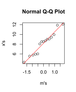
i) For the Q-Q plot, we just need to plot \(\hat {m}_j\) versus \(x_{(j)}\). The graph obtained is presented below:
-
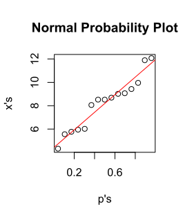
ii) For the alternative Q-Q plot, we just need to plot \(P_j\) versus \(x_{(j)}\). The graph obtained is presented below:
-
iii) Finally, the P-P plot is obtained by plotting \(\hat {P}_j\) versus \(x_{(j)}\). The graph obtained is presented below:
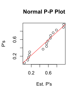
The three graphical procedures presented graphs with a good fit of the least squares line to the dispersion of points in each case, indicating, visually (hence subjectivity) that there are no normality departures. The R functions are presented in the sequence:
# Function to obtain the normal Q-Q plots # and rQ, normal quantil-quantil correlation normQQPlot <- function(x) { n <- length(x) Pj <- ((1:n)-0.375) / (n + 0.25) mj <- qnorm(Pj) Xj <- sort(x) par(mfrow = c(1, 2)) plot(mj, Xj, xlab="m's",ylab="x's", main="Normal Q-Q Plot") abline(lm(Xj~mj),col="red") ######## Normal Probability Plot ##### plot(Pj, Xj, xlab="p's",ylab="x's", main="Normal Probability Plot") abline(lm(Xj~Pj),col="red") rQ <- cor(Xj,mj) return(list(rQ=rQ)) } # Function to obtain the normal P-P plots # and rQ, normal quantil-quantil correlation normPPPlot <- function(x) { n <- length(x) Pj <- ((1:n)-0.375) / (n + 0.25) Xj <- sort(x) Sn <- sqrt(var(x) * (n - 1) / n) Phj <- pnorm((Xj -mean(x))/Sn) plot(Phj, Pj, xlab="Est. P's",ylab="P's", main="Normal P-P Plot") abline(lm(Pj~Phj),col="red") } # Example: Exercise 10.5.1 x <- c(8.52,9.07,11.90,9.43,4.32, 5.77,8.52,5.95,5.56,9.02, 12.08,8.06,9.96,6.02,8.69) normQQPlot(x) normPPPlot(x) -
-
10.2.2 Let us repeat the previous process for the new data set. We will choose the most appropriate procedures and provide fewer details of the calculations performed, since most of the necessary details have already been presented in the previous exercise.
-
a) Chi-square test:
The frequency distribution is presented below, including the expected frequencies by the normal model considering a mean of 3.8397 and standard deviation of 3.3154 (values estimated in the sample):
-----------------------------------------------------------------------
Classes (i)       Class midpoint X(i)   FO(i)    FE(i)
-----------------------------------------------------------------------
[-0.9268, 1.5286)     0.3009           12     9.7140
[ 1.5286, 3.9841)     2.7564           13    10.9798
[ 3.9841, 6.4396)     5.2119            7    10.6467
[ 6.4396, 8.8951)     7.6673            6     6.1125
[ 8.8951,11.3506)    10.1228            1     2.0763
[11.3506,13.8060)    12.5783            1     0.4697
-----------------------------------------------------------------------
The value of the test statistic is:
\(\seteqnumber{0}{10.}{0}\)\begin{align*} \chi ^2_c =& \sum _{i=1}^{k} \dfrac {\left (F_i-FE_i\right )^2}{FE_i}= \sum _{i=1}^{6} \dfrac {\left (F_i-FE_i\right )^2}{FE_i}\\ =& \dfrac {(12-9.7140)^2}{9.7140}+\dfrac {(13-10.9798)^2}{10.9798} + \dfrac {(7-10.6467)^2}{10.6467}+ \\ & \,\, +\dfrac {(6-6.1125)^2}{6.1125}+ \dfrac {(1-2.0763)^2}{2.0763}+\dfrac {(1-0.4697)^2}{0.4697}\\ =& 3.3175. \end{align*}
The tabulated value is \(\chi ^2_{0.975;\nu =4}\) \(=\) 11.1433. Thus, since the calculated chi-square value is less than the tabulated one, there is no significant evidence to reject the null hypothesis. This test generally has a very weak performance, presenting high rates of type I and II errors. In this case, the data were simulated from an exponential population and the null hypothesis of normality, which is false, should be rejected. It was not, indicating that there was a type II error.
-
b) Using the option of Royston (1993), we obtained \(W\) \(=\) 0.8656 and \(p\)-value \(=\) 0.00022. Since the \(p\)-value is less than the nominal level of \(5\%\), we must reject the null hypothesis of normality. The result led to a correct decision and was contrary to the decision of the chi-square test, which as we said before has low performance.
-
c) The Q-Q plot correlation was \(r_Q\) \(=\) 0.9335. The tabulated value for \(\alpha \) \(=\) \(5\%\) and \(n\) \(=\) \(40\) is 0.9726. Since the calculated value is less than the tabulated value, we must reject the hypothesis of normality at the nominal significance level of \(5\%\). This result agrees with that of the Shapiro-Wilk test and disagrees with that of chi-square.
The graphical procedures provided the following results:
-
i) Q-Q plot and normal probability graphs:
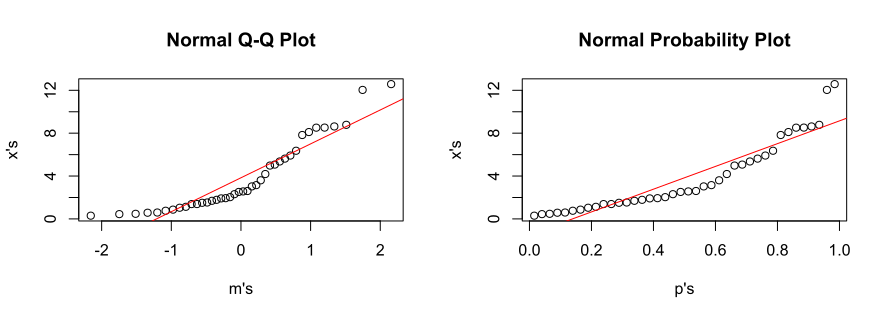
There is an indication of non-normality of the data.
-
ii) P-P plot:
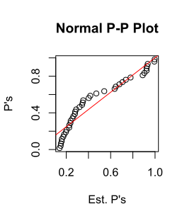
There is an indication of non-normality of the data.
The comparison with the results of the skewness and kurtosis tests of example 10.5 of the Book indicates that the different tests agree with each other. The exception was with the chi-square test. The data set and the call of the appropriate functions is presented below so that the reader can reproduce these results or even use another database of interest.
# Example 10.5 from the book x <-c(8.5209, 4.1871, 2.5163, 1.9133, 8.7796, 5.9117, 0.7608, 12.0372, 5.6255, 6.3604, 5.0679, 3.0310, 1.1281, 1.3850, 12.5783, 2.0292, 3.6014, 7.8288, 1.3829, 1.9344, 0.8642, 8.5144, 4.9774, 0.5759, 1.0414, 0.3009, 1.7809, 2.5638, 5.3587, 2.3066, 1.5298, 8.1052, 2.6035, 0.5953, 1.5033, 3.1507, 1.6889, 0.4451, 0.4750, 8.6276) normQQPlot(x) normPPPlot(x) -
-
10.2.3 The maximum likelihood estimator of the parameter \(\lambda \) of the exponential model is \(1/\bar {X}\). Although the use of the maximum likelihood estimate is suggested, which in this case is \(1/\bar {X}\) \(=\) 1/3.83971 \(=\) 0.2604363, we know that correlation is a quantity that is invariant to scale changes and, therefore, we do not need to use this quantity. If, for example, \(Y\sim \exp (1)\), then \(X\) \(=\) \(Y/\lambda \), \(\lambda >0\), has an exponential distribution with parameter \(\lambda \), that is, \(X\) \(\sim \) exponential\((\lambda )\), which we can easily prove using the Jacobian method of the transformation. Thus, the scale change does not influence the distribution and, therefore, we can simulate from a standard exponential distribution \((Y\sim \textrm {exp}(\lambda ))\), since the correlation \(r_Q\) will not be affected by the simple scale change, when we consider an exponential with parameter \(\lambda \), of any exponential variable \(X\).
-
(a) The proposal of the test is:
-
i) we compute \(p_j\) \(=\) \((j-0.375)/n(+0.25)\) for all \(j=1\), \(2\), \(\cdots \), \(n\);
-
ii) we sort the values of \(x\), \(x_{(j)}\), \(j=1\), \(2\), \(\cdots \), \(n\);
-
iii) we estimate the mean of the order statistics of the exponential by \(m_j\) \(=\) \(F_Y^{-1}(p_j)\), where \(F_Y^{-1}\) is the inverse distribution function of an exponential with \(\lambda =1\), considering that \(Y\) \(\sim \) exponential\((1)\), for all \(j=1\), \(2\), \(\cdots \), \(n\);
-
iv) we compute the sample correlation \(r_Q\) between \(p_j\) and \(m_j\);
-
v) we plot \(m_j\) (on the abscissa) versus \(x_{(j)}\) (on the ordinate) to obtain the Q-Q plot;
-
vi) we simulate data from the exponential distribution with \(\lambda =1\) and the same sample size as the original sample. We repeat, for each simulated sample, steps (ii), (iii) and (iv), with the same values of \(p_j\)’s from step (i) and store the values of \(r_Q\)’s obtained. We denote these simulated values by \(r_{Q_i}\), for all \(i=1\), \(2\), \(\cdots \), \(N\);
-
vii) we calculate the \(p\)-value by
\(\seteqnumber{0}{10.}{0}\)\begin{align*} \textrm {$p$-value} =& \dfrac {\displaystyle \sum _{i=1}^{N} I(r_{Q_j}\le r_Q)}{N}, \end{align*} where \(I()\) is the indicator function. We choose \(N\) as being at least equal to \(1000\) Monte Carlo simulations;
-
viii) we return \(r_Q\) and the \(p\)-value.
Since the procedure is essentially computational, we developed an R function to perform this task.
# Function to obtain the Q-Q plot for exponential
# distribution and to apply the Q-Q plot
# correlation test
expQQrQTest <- function(x, N = 10000)
{
  n <- length(x)
  pj <- ((1:n)-0.375) / (n + 0.25)
  mj <- qexp(pj)
  xj <- sort(x)
  plot(mj, xj, xlab="m's",ylab="x's",
       main="Exponential Q-Q Plot")
  abline(lm(xj~mj),col="red")
  rQ <- cor(xj,mj)
  randomrQ <- function(n, pj)
  {
    xs <- rexp(n)
    msj <- qexp(pj)
    xsj <- sort(xs)
    rQs <- cor(xsj,msj)
    return(rQs)
  }
  nullRqDist <- matrix(c(n), N, 1)
  nullRqDist <- apply(nullRqDist,1,randomrQ,pj)
  p.value <- length(nullRqDist[nullRqDist<=rQ])/N
  return(list(rQ = rQ, p.value=p.value))
}

# Example 10.5 from the book
x <-c(8.5209, 4.1871, 2.5163, 1.9133, 8.7796, 5.9117, 0.7608, 12.0372,
      5.6255, 6.3604, 5.0679, 3.0310, 1.1281, 1.3850, 12.5783, 2.0292,
      3.6014, 7.8288, 1.3829, 1.9344, 0.8642, 8.5144, 4.9774, 0.5759,
      1.0414, 0.3009, 1.7809, 2.5638, 5.3587, 2.3066, 1.5298, 8.1052,
      2.6035, 0.5953, 1.5033, 3.1507, 1.6889, 0.4451, 0.4750, 8.6276)
N <- 10000
expQQrQTest(x, N)
Considering \(N\) \(=\) \(10000\) simulations for this case, we obtained \(r_Q\) \(=\) 0.9967996 and \(p\)-value \(=\) 0.5283. Thus, considering the nominal significance level of \(5\%\) we should not reject the hypothesis of exponential distribution for the data set in question. We know that these data were simulated from an exponential distribution and, therefore, the result confirms what we already knew previously. The Q-Q plot graph of this case is:
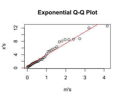
We can observe that there is a good fit of the least squares line to the dispersion of points, which indicates that the exponential distribution is adequate for this case. Note that we made this same Q-Q plot for this data set in the previous exercise, considering as null hypothesis that the data were normal. The result was that the normality hypothesis (visually and subjectively) should be rejected.
-
-
(b) We performed Monte Carlo simulations in two ways: i) considering data from an exponential with parameter \(\lambda \) and sample of size \(n\). Since the correlation is invariant with respect to the change of \(\lambda \), only the value of \(n\) was changed. Thus, we simulated data with \(\lambda =2\) and \(n\) \(=\) \(5\), \(50\), \(100\) and \(1000\); b) we considered samples from the standard normal, with the same values of \(n\) as before. In both cases \(N=2000\) values were used to obtain the \(p\)-values.
The proportion of rejections of \(H_0\) were computed in both cases in \(M=2000\) Monte Carlo simulations. In the first case, situation (a), the rejections indicate the type I error rates and in the second case, situation (b), the power of the test. The results are presented in the following table only for the level \(\alpha \) \(=\) 0.05 of significance:
\(n\) Exponential\((\lambda =2)\) Standard Normal 5 0.0515 0.1895 50 0.0450 0.9620 100 0.0500 1.0000 1000 0.0515 1.0000 The results show that the test adequately controls the type I error rate and has high power. The small differences from the value of \(5\%\) are attributed to the Monte Carlo error. Of course we restricted our power study to only one distribution, the normal. A broader study would involve many significance levels, but values of \(n\) and other distributions under the alternative hypothesis.
-