Basic Statistics
9.2 Solutions
-
9.2.1 The confidence interval for the mean zinc content \(\mu \) in ppm is given by:
\(\seteqnumber{0}{9.}{0}\)\begin{align*} CI_{1-\alpha }(\mu ):& \bar {X} \pm t_{\alpha /2;\nu =99} \dfrac {S}{\sqrt {n}}\\ & =700 \pm 1.984 \times \sqrt {\dfrac {400}{100}}\\ & =700\pm 3.968\\ & =[696.03,\,\, 703.97]. \end{align*}
Thus, we can state, with \(95\%\) confidence, that the true mean \(\mu \) of zinc content in the chemical constitution of the chickens that received a zinc-based diet (mineral supplement in the feed) should be a value between 696.03 ppm and 703.97 ppm. Since the value of \(400\) ppm of the chickens that do not receive the mineral supplementation does not belong to the confidence interval, we can say that there is a significant effect \((P<\)0.05\()\) on the mean zinc content when the animals are submitted to a diet with mineral supplementation.
-
9.2.2 The sample mean and variance are \(\bar {X}\) \(=\) \(12\) and \(S^2\) \(=\) 13.6, respectively. The sample size is \(n\) \(=\) \(61\) and the required upper quantiles of the Student’s \(t\) distribution are \(t_{0.025;\nu =99}\) \(=\) 2.000 and \(t_{0.005;\nu =99}\) \(=\) 2.660. The \(95\%\) and \(99\%\) intervals are:
\(\seteqnumber{0}{9.}{0}\)\begin{align*} CI_{0.95}(\mu ):& \bar {X} \pm t_{0.025;\nu =60} \dfrac {S}{\sqrt {n}}\\ & =12 \pm 2.000 \times \sqrt {\dfrac {13.6}{61}}\\ & =12\pm 0.94\\ & =[11.06,\,\, 12.94] \end{align*} and
\(\seteqnumber{0}{9.}{0}\)\begin{align*} CI_{0.99}(\mu ):& \bar {X} \pm t_{0.005;\nu =60} \dfrac {S}{\sqrt {n}}\\ & =12 \pm 2.660 \times \sqrt {\dfrac {13.6}{61}}\\ & =12\pm 1.26\\ & =[10.74,\,\, 13.26]. \end{align*} We verify, as expected by theory, that the larger the sample size, the greater the amplitude of the confidence interval (less precise). This is due to the fact that with the same resources (same sample and same estimates), an increase in confidence must provide an increase in amplitude so that the probability of greater coverage with a greater nominal confidence can be achieved. Thus, we should remember that we will always be penalized with an adverse effect when we have the same resources but want to guarantee greater confidence. For this reason we cannot increase the confidence coefficient to a number very close to \(100\%\), because we would have useless confidence intervals. An example would be to state that the true mean milk production is a value between \(0\) and \(\infty \) liters, with \(100\%\) confidence. Of course this is an extreme case to reinforce the idea of the usefulness of the interval. On the other hand, we cannot seek an interval that is useful but with very low confidence (close to zero).
-
9.2.3 The sample total is \(k\) \(=\) \(n\bar {X}\) \(=\) \(10\times \)19.6 \(=\) \(196\). The exact interval for \(\mu \) \(=\) \(\lambda \), which explores the relationship between the Poisson and gamma (or chi-square) distribution, is given by
\(\seteqnumber{0}{9.}{0}\)\begin{align*} CI_{1-\alpha }(\mu ): & \left [\lambda _I =\dfrac {\chi ^2_{1-\alpha /2;\,\nu =2k}}{2n},\,\, \lambda _S =\dfrac {\chi ^2_{\alpha /2;\,\nu =2k+2}}{2n}\right ]\\ :&\left [\dfrac {\chi ^2_{0.975;\,\nu =392}}{20},\,\, \dfrac {\chi ^2_{0.025;\,\nu =392+2}}{20}\right ]\\ :&\left [\dfrac {339.0392}{20},\,\, \dfrac {450.8879}{20}\right ]\\ :& [16.9520,\,\,22.5444]. \end{align*}
The first interval based on a normal approximation is
\(\seteqnumber{0}{9.}{0}\)\begin{align*} CI_{1-\alpha }(\mu ): & \left [\bar {X}-Z_{0.025} \sqrt {\frac {\bar {X}}{n}},\,\, \bar {X}+Z_{0.025} \sqrt {\frac {\bar {X}}{n}}\right ]\\ :& \left [19.6-1.96\sqrt {\frac {19.6}{10}},\,\, 19.6+1.96 \sqrt {\frac {19.6}{10}}\right ]\\ :& [16.8561,\,\,22.3440]. \end{align*}
The second interval based on a normal approximation is
\(\seteqnumber{0}{9.}{0}\)\begin{align*} CI_{1-\alpha }(\mu ): & \left [\frac {1}{4}\left (\frac {Z_{0.025}}{\sqrt {n}}- \sqrt {\frac {Z_{0.025}^2}{n}+4\bar {X}}\right )^2,\,\, \frac {1}{4}\left (\frac {Z_{0.025}}{\sqrt {n}}+ \sqrt {\frac {Z_{0.025}^2}{n}+4\bar {X}}\right )^2\right ]\\ :& \left [\frac {1}{4}\left (\frac {1.96}{\sqrt {10}}- \sqrt {\frac {1.96^2}{10}+4\times 19.6}\right )^2,\,\, \frac {1}{4}\left (\frac {1.96}{\sqrt {10}}+ \sqrt {\frac {1.96^2}{10}+4\times 19.6}\right )^2\right ]\\ :& [17.0414,\,\,22.5427]. \end{align*}
In this case, the confidence interval for the mean number of leaf-cutter ant nests per 0.5 hectare. The limits for nests per hectare can be obtained by multiplying by \(2\) the limits previously obtained in each case. The values of both approximations were very close to the exact limits and can be good alternatives to be used. The second approximation provides slightly better results.
The exact confidence interval, based on the sampling unit of \(1\) ha, is:
\(\seteqnumber{0}{9.}{0}\)\begin{align*} CI_{1-\alpha }(\mu ): & [33.9040,\,\, 45.0888]. \end{align*} Thus, we have that the mean number of nests per hectare should be a value between 33.9040 and 45.0888, with \(95\%\). If the cost to extinguish one nest, then the mean cost of extinguishing all nests per hectare is 17.55 reais, with 95% confidence, should be between 595.01 and 791.31 reais on average per ha. If there are \(100,000\) ha, the company should make a disbursement between 59.50 and 79.13 million, with \(95\%\) confidence.
-
9.2.4 Obtain the approximate and exact confidence intervals for the mean of the exponential. We have two approximations, one specific for the exponential and another, general, using the central limit theorem. The sample mean is \(\bar {X}\) \(=\) 98.3033 obtained from the sample of size \(n=30\). The exact interval is:
\(\seteqnumber{0}{9.}{0}\)\begin{align*} CI_{1-\alpha }(\mu ): & \left [\frac {2n\bar {X}}{\chi ^2_{\alpha /2,\nu =2n}},\,\, \frac {2n\bar {X}}{\chi ^2_{1-\alpha /2;\nu =2n}}\right ]\\ :& \left [\frac {2\times 30\times 98.3033}{83.29767},\, \frac {2\times 30\times 98.3033}{40.48175}\right ]\\ & =\left [70.8087,\, 145.7002\right ]. \end{align*}
The classical normal approximation, using the central limit theorem, is:
\(\seteqnumber{0}{9.}{0}\)\begin{align*} CI_{95\%}(\mu ):& \bar {X} \pm t_{\alpha /2; \nu =n-1} \frac {S}{\sqrt {n}}\\ :& 98.3033\pm 2.04523\times \frac {80.88364}{\sqrt {30}}\\ :& \left [68.1009,\, 128.5058\right ]. \end{align*}
Finally, the confidence interval developed in the Book is:
\(\seteqnumber{0}{9.}{0}\)\begin{align*} CI_{1-\alpha }(\mu ): & \left [\frac {\bar {X}\sqrt {n}}{\sqrt {n}+ Z_{\alpha /2}},\,\, \frac {\bar {X}\sqrt {n}}{\sqrt {n}-Z_{\alpha /2}}\right ]\\ :& \left [\frac {98.3033\sqrt {30}}{\sqrt {30}+ 1.96},\,\, \frac {98.3033\sqrt {30}}{\sqrt {30}-1.96}\right ]\\ :& \left [72.3969,\, 153.0820\right ]. \end{align*}
The classical normal approximation was the one that presented the worst result among the two approximations presented. Obviously, in real situations, if we have an exact theory we should always or almost always opt for it. There may be some exception, provided it is scientifically justified, such as, for example, an approximate confidence interval that returns shorter intervals and maintains the nominal confidence for most cases relative to the sample sizes.
-
9.2.5 For the data of exercise 9.2.3, the bootstrap intervals are presented below:
Method
LL UL Standard
16.7270 22.4808 Standard with bias correction
16.8658 22.3346 Percentile
16.8000 22.8000 Basic (Hall, 1992)
16.7000 22.2000 Bias Correction
17.0000 22.7000 Student’s \(t\)
16.8600 24.8100 The results were very similar, except for the upper limit for the Student’s \(t\) interval. Since the procedures are essentially computational, we present below an R program with our implementation, which also contains codes for the intervals of the boot package of R. Thus, the reader can reproduce their own results, use other functions and other data sets of interest. It should be emphasized that the BCA method of R, package boot, differs from the method presented, by incorporating an acceleration of the bias correction. See details in Ferreira (2013).
# Program to Apply the bootstrap CIs of chapter 9

# function to do 1 bootstrap resampling and return an estimate
# est is function of the estimator, a: is an artifice-not used
bootstrap <- function(a, x, est, ...)
{
  n   <- length(x)
  xb <- sample(x, n, replace = TRUE)
  est.boot <- est(xb)
  return(est.boot)
}

# function to obtain the bootstrap distribution
distboot <- function(B = 2000, x, est, ...)
{
  a <- as.matrix(1:B, B, 1)
  result <- apply(a, 1, bootstrap, x, est)
  plot(hist(result))
  return(result)
}

# Function to obtain the standard error of the estimator of interest
serrboot <- function(B = 2000, x, est, ...)
{
  result <- distboot(B, x, est)
  se.boot <- sd(result)
  est.boot <- est(x)
  return(list(est = est.boot, se = se.boot))
}

# receives the original sample and returns
# the standard confidence interval with or without
# bias correction
CI.boot.standard <- function(B = 2000, x,
                            est, alpha=0.05, CV = TRUE)
{
  result <- distboot(B, x, est)
  est.boot <- est(x)
  se.boot <- sd(result)
  mean.boot <- mean(result)
  bias.boot <- mean.boot - est.boot
  if (CV == TRUE)
  {
    LL <- est.boot - bias.boot + qnorm(alpha/2)*se.boot
    UL <- est.boot - bias.boot+ qnorm(1-alpha/2)*se.boot
  } else
  {
    LL <- est.boot + qnorm(alpha/2)*se.boot
    UL <- est.boot + bias.boot+ qnorm(1-alpha/2)*se.boot
  }
  return(list(est = est.boot, se =se.boot,
              Li= LL, Ls = UL))
}

# receives the original sample and returns
# the percentile confidence interval
CI.boot.percent <- function(B = 2000, x, est, alpha=0.05, ...)
{
  result <- distboot(B, x, est)
  result <- sort(result)
  est.boot <- est(x)
  se.boot <- sd(result)
  k1 <- trunc((B+1)*alpha/2)
  if (k1 <= 0) k1 <- 1
  k2 <- trunc((B+1)*(1-alpha/2))
  LL <- result[k1]
  UL <- result[k2]
  return(list(est = est.boot, se =se.boot,
              Li= LL, Ls = UL))
}

# receives the original sample and returns
# the basic confidence interval of Hall(1992)
CI.boot.basic <- function(B = 2000, x, est, alpha=0.05)
{
  result <- distboot(B, x, est)
  result <- sort(result)
  est.boot <- est(x)
  se.boot <- sd(result)
  k1 <- trunc((B+1)*alpha/2)
  if (k1 <= 0) k1 <- 1
  k2 <- trunc((B+1)*(1-alpha/2))
  LL <- 2*est.boot - result[k2]
  UL <- 2*est.boot - result[k1]
  return(list(est = est.boot, se =se.boot,
              Li= LL, Ls = UL))
}
# receives the original sample and returns # the confidence interval with bias correction CI.boot.BC <- function(B = 2000, x, est, alpha=0.05, ...) { result <- distboot(B, x, est) result <- sort(result) est.boot <- est(x) se.boot <- sd(result) k1 <- sum(result < est.boot) / B z0 <- qnorm(k1) za2 <- qnorm(alpha/2) p1 <- pnorm(2*z0 + za2) k1 <- trunc((B+1) * p1) if (k1 <= 0) k1 <- 1 z1a2 <- qnorm(1-alpha/2) p2 <- pnorm(2*z0 + z1a2) k2 <- trunc((B+1) * p2) LL <- result[k1] UL <- result[k2] return(list(est = est.boot, se =se.boot, Li= LL, Ls = UL)) } # Example Book 9.1.5 #x <- c(391.1, 98.3, 197.3, 77.5, 26.5, # 92.4, 30.3, 199.8, 99.9, 31.2, # 32.2, 78.7, 16.7, 55.4, 213.3, # 164.7, 37.1, 15.2, 41.7, 201.9, # 56.8, 96.5, 38.0, 104.1, 78.5, # 35.0, 95.8, 108.2, 78.6, 156.4) x <- c(20, 16, 24, 18, 23, 19, 16, 14, 16, 30) # function for the mean B <- 2000 alpha = 0.05 est.mean <- function(x) mean(x) alpha = 0.05 est <- est.mean CI.boot.standard(B, x, est, alpha, FALSE) CI.boot.standard(B, x, est, alpha) CI.boot.percent(B, x, est, alpha) CI.boot.basic(B, x, est, alpha) CI.boot.BC(B, x, est, alpha) # Using R functions library(boot) # this library must be installed samplemean <- function(x, d) { m <- mean(x[d]) n <- length(d) v <- (n-1) * var(x[d]) / n^2 return(c(m, v)) } CIboot2 <- boot(x, samplemean, R = 1999) boot.ci(CIboot2, conf = 0.95, type = c("norm","basic", "perc", "bca", "stud")) print(sd(CIboot2$t[,1])) -
9.2.6 The hypothesis of interest is given by:
\(\seteqnumber{0}{9.}{0}\)\begin{align*} H_0:\, \mu =& 3.21 &\textrm { vs }&& H_1:\, \mu \ne & 3.21. \end{align*}
The sample mean and variance are
\(\seteqnumber{0}{9.}{0}\)\begin{align*} \bar {X}=& 3.10 &\textrm { and }&& S^2=& 0.80, \end{align*} in a sample of size \(n=20\) animals. We set the nominal significance level at 0.05 and compute the test statistic
\(\seteqnumber{0}{9.}{0}\)\begin{align*} t_c=& \dfrac {\bar {X}-\mu _0}{\dfrac {S}{\sqrt {n}}} =\dfrac {3.10-3.21}{\sqrt {\dfrac {0.80}{20}}}=-0.55. \end{align*}
The critical region (region of rejection of the null hypothesis), knowing that \(t_{0.025; \nu =19}=\)2.093, is given by:
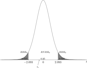
Since the value of \(t_c\) belongs to the non-rejection region of the hypothesis, by the \(t\) test, with \(95\%\) confidence, the null hypothesis should not be rejected, that is, we conclude that phlorizin does not have a mean glucose different from the mean of untreated animals, having no effect on the mean arterial glucose of the animals.
-
9.2.7 If the data are Poisson \((\lambda )\), then we know that the sum of the \(n\) variables of a random sample is also Poisson with parameters \(n\lambda \). If we use the relationship of the Poisson with the gamma, we have
\(\seteqnumber{0}{9.}{0}\)\begin{align*} F_X(x;\lambda ) =& 1-I_{\lambda }(x+1), \end{align*} where \(F_X(x;\lambda )\) is the distribution function of a variable \(X\) \(\sim \) Poisson\((\lambda )\) and \(I_{\lambda }(x+1)\) is the distribution function of a gamma with parameter \(x+1\) evaluated at \(\lambda \), that is, \(G(\lambda ; x+1)\), where \(G\) is the distribution function of the gamma.
Thus, we can apply the required test in two ways. First, if we perform the \(95\%\) exact confidence interval for the mean of the Poisson, which in this case is [3.98, 5.97], and evaluate whether the hypothesized value \(\lambda _0\) is or is not contained in the interval. In this case, we state, by hypothesis, that the mean in \(10000\) m\(^2\) is equal to \(121\). This is equivalent to the mean in the area of \(500\) m\(^2\) to a mean value of 6.05, which is \(\lambda _0\). Thus, since the value 6.05 does not belong to the generated interval, we must reject the null hypothesis.
The second alternative is to use the exact relationship above, between the Poisson and the gamma. The procedure we must follow follows the following steps (theory not presented in the Book), in which we include the results of the specific case at each step (mixing theory and practice simultaneously).
The hypothesis of interest is given by:
\(\seteqnumber{0}{9.}{0}\)\begin{align*} H_0:\, \lambda =& \lambda _0 &\textrm { vs }&& H_1:\, \lambda \ne & \lambda _0, \end{align*} which in this case is
\(\seteqnumber{0}{9.}{0}\)\begin{align*} H_0:\, \lambda =& 6.05 &\textrm { vs }&& H_1:\, \lambda \ne & 6.05, \end{align*} where \(\lambda _0\) \(=\) \(121/20\) \(=\) 6.05. The value \(20\) refers to the transformation constant of the areas of each sampling unit of \(500\) m\(^2\) to hectare, \(10000\) m\(^2\).
If \(Y\) \(=\) \(\sum _{j=1}^{n} X_i\) is the Poisson sum, we know that, under \(H_0\), \(Y\) \(\sim \) Pois\((n\lambda _0)\). Thus we must compute this sum, which in this case has a realization of \(98\). If \(H_0\) is true, we must reject \(H_0\) if
\(\seteqnumber{0}{9.}{0}\)\begin{align*} F_Y(y;n\lambda _0)\le \alpha /2 &\textrm { or }&& 1 - F_Y(y-1;n\lambda _0)\le \alpha /2. \end{align*} An alternative to this criterion is to use the approximate calculation of the \(p\)-value, using the relationship of the Poisson with the gamma, by
\(\seteqnumber{0}{9.}{0}\)\begin{align*} \textrm {$p$-value}=& 2\min (1-I_{n\lambda _0}(y+1), I_{n\lambda _0}(y)). \end{align*}
For this case, with \(n=20\) and \(y=98\), we have that the \(p\)-value \(=\) \(2\min (\)0.0179, 0.9860\()\) \(=\) 0.0358. Thus, at the nominal significance level \(\alpha \) \(=\) 0.05, we must reject \(H_0\) and we can state that the mean number of bromeliad plants per hectare is less than \(121\). We have that the confidence interval for plants/ha is given by [89.6, 119.4] (limits obtained by multiplying the limits of the previous interval by \(20\)).
We made an R program to facilitate the application of the test, which is presented below:
# Exact test for Poisson # H_0: lambda = lambda_0 # sum(x)~sim(nlambda_0) under H_0 pois.test <- function(x, lambda0) { n <- length(x) y <- sum(x) xb <- y / n p1 <- 1 - pgamma(n*lambda0, y + 1) p2 <- pgamma(n*lambda0, y) p.value <- 2 * min(p1, p2) return(list(mean = xb, p.value=p.value)) } # number of bromeliads per 500m2 # proportionality constant # is 20 (20*x: number per ha) x<-c(1, 6, 6, 6, 7, 2, 7, 6, 6, 3, 3, 10, 4, 3, 7, 3, 5, 4, 4, 5) pois.test(x, 6.05) # 121/20=6.05 -
9.2.8 To determine the sample size to estimate the mean \(\mu \) of a normal population relative to yield with an error of \(200\) kg and \(95\%\) confidence, we need a pilot sample or an estimate of the variance. In this case, we have an estimate of the population variance given by \(S^2\) \(=\) 1.4 \(t^2\)/ha. Thus, we must solve iteratively the following expression, knowing that the error upward and downward in tons per hectare is 0.2 t/ha:
\(\seteqnumber{0}{9.}{0}\)\begin{align*} n =& \dfrac {S^2t_{\alpha /2; \nu =n-1}^2}{e^2}. \end{align*}
We start with an initial estimate of \(n\) of any value, for example, \(n=10\). Thus, the tabulated value of \(t\) is \(t_{0.025;\nu =9}\) \(=\) 2.262157. Thus, in the first iteration we have
\(\seteqnumber{0}{9.}{0}\)\begin{align*} n =& \dfrac {1.4\times 2.262157^2}{0.2^2}=179.11. \end{align*} Since the value is different from the previous value \(n=10\), we must repeat the process. Thus, we round \(n\) to \(n=179\) and determine \(t_{0.025;\nu =178}\) \(=\) 1.973381. Therefore, the new value of \(n\) is
\(\seteqnumber{0}{9.}{0}\)\begin{align*} n =& \dfrac {1.4\times 1.973381^2}{0.2^2}=136.2981. \end{align*} Since the value is different from the previous value \(n=179\), we must repeat the process. Thus, we round \(n\) to \(n=136\) and determine \(t_{0.025;\nu =135}\) \(=\) 1.977692. Therefore, the new value of \(n\) is
\(\seteqnumber{0}{9.}{0}\)\begin{align*} n =& \dfrac {1.4\times 1.977692^2}{0.2^2}=136.8943. \end{align*} Since the rounded value 137 is different from the previous value \(n=136\), we must repeat the process. Thus, we round \(n\) to \(n=137\) and determine \(t_{0.025;\nu =136}\) \(=\) 1.977561. Therefore, the new value of \(n\) is
\(\seteqnumber{0}{9.}{0}\)\begin{align*} n =& \dfrac {1.4\times 1.977561^2}{0.2^2}=136.8761. \end{align*} Since the rounded value is equal to the value of the previous step, we have that the sample size necessary to estimate the mean yield with error upward and downward of 0.2 t/ha and \(95\%\) confidence is \(n=137\) sampling units.
We present the R program below to perform this process automatically in an easier way.
# Function to determine the sample size for # estimating mu from normal population with # confidence 1-alpha, error margin "e" and # estimate of sig^2 (S2) SampleSizeEstMu <- function(e, S2, alpha=0.05, n0 = 10) { it <- 0 print("Iterations") print(c(" It # "," t tab."," n")) repeat { n <- n0 ta <- qt(1 - alpha/2, n - 1) n0 <- (S2 * ta^2 / e^2) it <- it + 1 print(c(it,ta,n0)) if (abs(n0 - n) < 1) { n0 <- round(n0) break } if (it >= 1000) break } return(list(n = round(n0), it = it)) } # Example 9.6.8 e <- 0.2 s2 <- 1.4 alpha <- 0.05 SampleSizeEstMu(e, s2, alpha) -
9.2.9 To determine the sample size we will use the approximate formula given by
\(\seteqnumber{0}{9.}{0}\)\begin{align*} n=& \dfrac {S^2\left (t_{\beta ;\nu }+t_{\alpha /2;\nu }\right )^2}{\delta ^2}, \end{align*} where \(\delta \) is the minimum significant difference \(\delta \) \(=\) \(|\mu _0-\mu |\). Again, since the value of \(n\) is implicit (degrees of freedom of the quantiles of the Student’s \(t\) distribution), the expression must be solved iteratively and for this we must consider any initial value for the sample size, which in this case will be \(n=10\). The value of the estimate of the population standard deviation in the pilot sample performed was \(s^2\) \(=\) 0.56 t/ha.
-
a) In this case we have, \(1-\beta \) \(=\) 0.95, \(1-\alpha \) \(=\) 0.95 and \(\delta \) \(=\) 0.2 t/ha. We have, with \(n=10\), that \(t_{\beta ;\nu }\) \(=\) \(t_{0.05;9}\) \(=\) 1.833113 and \(t_{\alpha /2;\nu }\) \(=\) \(t_{0.025;9}\) \(=\) 2.262157. Therefore,
\(\seteqnumber{0}{9.}{0}\)\begin{align*} n=& \dfrac {S^2\left (t_{\beta ;\nu }+ t_{\alpha /2; \nu }\right )^2}{\delta ^2}= \dfrac {0.56^2\left (1.833113+ 2.262157\right )^2}{0.2^2}\\ =& 131.486499 . \end{align*} Since this value differs from the initial value \(10\), we must repeat. We determine the new quantiles of the \(t\) distribution and determine the new value of \(t\) and compare with this last one. If there is convergence, on the integer scale, we stop the process. Otherwise we redo the process. We did this using the R program below. The results (without rounding) of the iterative process are:
Iterations \(t_{\alpha /2; \nu }\) \(t_{\beta ;\nu }\) \(n\) 1 2.262157 1.833113 131.486499 2 1.978311 1.656615 103.587477 3 1.983359 1.659843 104.059687 4 1.983250 1.659774 104.049534 Since the final rounded value is equal to the value of the previous step also rounded, we have that the sample size necessary to estimate the mean yield with minimum significant difference of 0.2 t/ha, \(95\%\) confidence and power of \(95\%\) is \(n=104\) sampling units.
We present the R program below to perform this process automatically in an easier way, as in the previous exercise.
# Function to determine the sample size for # testing H_0: mu = mu_0, considering samples # from normal population with # confidence 1-alpha, probability of type II error # beta, lsd "d" and estimate of sig^2 (S2) SampleSizeTestMuBilat <- function(d, S2, alpha=0.05, beta = 0.05, n0 = 10) { it <- 0 print("Iterations") print(c(" It # "," ta "," tb "," n")) repeat { n <- n0 ta <- qt(1 - alpha/2, n - 1) tb <- qt(1 - beta, n - 1) n0 <- S2 * (ta + tb)^2 / d^2 it <- it + 1 print(c(it, ta, tb, n0)) if (abs(n0 - n) < 0.1) { n0 <- round(n0) break } if (it >= 1000) break } return(list(n = round(n0), it = it)) } # Example 9.6.9 (a) d <- 0.2 S2 <- 0.56^2 alpha <- 0.05 beta <- 0.05 n0 <- 10 SampleSizeTestMuBilat(d, S2, alpha, beta, n0) -
b) The power to detect a minimum difference of \(\delta =\)0.1 t/ha with confidence coefficient of \(95\%\) and \(n=104\) is obtained by:
\(\seteqnumber{0}{9.}{0}\)\begin{align*} t_{\beta ;\nu =103} =& \dfrac {\delta \sqrt {n}}{S}-t_{\alpha /2;\nu }= \dfrac {0.1\sqrt {104}}{0.56}-t_{0.025;103}\\ =& \dfrac {0.1\times 10.19804}{0.56}-1.983264\\ =& -0.1621857. \end{align*} Thus, the value of the upper quantile \(\beta \) of the \(t\) distribution is \(t_{\beta ;\nu =103}\) \(=\) \(-\)0.1621857. To determine \(\beta \), we can use the R command, \(1-pt(-0.1621857,103)\), which results in \(\beta \) \(=\) 0.5642613. Thus the power is \(1-\beta \) \(=\) 0.4357387, that is, the power is equivalent to 43.57%. In this formula we use an approximation, ignoring a part of an expression, to have a simplified solution. If we did not do so and solved the complete expression, we would have the exact power value given by 0.4358594, which is very close to the approximate solution. Therefore, we should not worry about using the approximation presented. We made a program to facilitate the obtaining by the reader for this case, which is presented below.
# Function to compute the power of t test for the # H_0: mu = mu_0, with d = mu - mu_0. PowerTestMuBilat <- function(d, S2, n, alpha=0.05) { ta <- qt(1 - alpha / 2, n - 1) q1 <- -ta - d * sqrt(n) / S2^0.5 q2 <- ta - d * sqrt(n) / S2^0.5 powExact <- pt(q1, n - 1) + (1 - pt(q2, n - 1)) powApprox <- 1 - pt(q2, n - 1) return(list(powExact = powExact, powApprox = powApprox)) } # Example 9.6.9 (b) d <- 0.1 S2 <- 0.56^2 alpha <- 0.05 n <- 104 PowerTestMuBilat(d, S2, n, alpha) -
c) To determine the minimum difference that will be detected with \(90\%\) power, confidence coefficient of \(95\%\) and \(n=104\) we use:
\(\seteqnumber{0}{9.}{0}\)\begin{align*} \delta =& \left (t_{\beta ;\nu }+t_{\alpha /2;\nu }\right ) \dfrac {S}{\sqrt {n}} = \left (1.289825+1.983264\right ) \dfrac {0.56}{\sqrt {104}}\\ =& 0.1797336 \textrm {t/ha.} \end{align*}
The R program to facilitate obtaining this value is presented below:
# Function to compute the lsd = d = mu - mu_0 of
# t test for the H_0: mu = mu_0, with alpha and beta.
LSDTestMuBilat <- function(S2, n, alpha=0.05, beta = 0.05)
{
  ta <- qt(1 - alpha / 2, n - 1)
  tb <- qt(1 - beta, n - 1)
  d <- (ta + tb) * S2^0.5 / sqrt(n)
  return(d)
}
# Example 9.6.9 (c)
S2 <- 0.56^2
alpha <- 0.05
beta <- 0.10
n <- 104
LSDTestMuBilat(S2, n, alpha, beta)
-
-
9.2.10 Confidence intervals for binomial proportions with \(n\) \(=\) \(500\) and number of successes \(y\) \(=\) \(6\). Let us obtain the exact interval and all approximations, including the approximation of Pratt (1968), which is the best known approximation. The point estimate is
\(\seteqnumber{0}{9.}{0}\)\begin{align*} \hat {p}=&\dfrac {y}{n}=\dfrac {6}{500}=0.0120=1.20\%. \end{align*}
-
a) Exact confidence interval
The value of the upper quantiles \(F_{0.025}\) with \(\nu _1\) \(=\) \(2(n-y+1)\) \(=\) \(2(500-6+1)\) \(=\) \(990\) and \(\nu _2\) \(=\) \(2y\) \(=\) \(2\times 6\) \(=\) \(12\) degrees of freedom and \(F_{0.025}\) with \(\nu _1\) \(=\) \(2(y+1)\) \(=\) \(2(6+1)\) \(=\) \(14\) and \(\nu _2\) \(=\) \(2(n-y)\) \(=\) \(2(500-6)\) \(=\) \(988\) degrees of freedom are 2.732611 and 1.878997, respectively. The exact interval is
\(\seteqnumber{0}{9.}{0}\)\begin{align*} CI_{1-\alpha }(p):& \left [\dfrac {1}{1+\frac {(n-y+1)F_{0.025;\nu _1 = 990,\nu _2=11}}{y}},\,\, \dfrac {1}{1+\frac {n-y}{(y+1) F_{0.025; \nu _1=14, \nu _2=988}}}\right ]\\ =& \left [\dfrac {1}{1+\frac {(500-6+1)\times 2.732611}{6}},\,\, \dfrac {1}{1+\frac {500-6}{(6+1)\times 1.878997}}\right ]\\ =& [0.004416172,\,\, 0.02593493]\\ =& \left [0.4416172\%,\,\, 2.593493\%\right ]. \end{align*}
-
b) Classical normal approximation:
\(\seteqnumber{0}{9.}{0}\)\begin{align*} CI_{0.95}(p):\,& \hat {p}\pm Z_{\alpha /2} \sqrt {\dfrac {\hat {p}(1-\hat {p})}{n}} = 0.0120 \pm 1.96 \sqrt {\dfrac {0.0120(1 - 0.0120)}{500}}\\ =& [0.2455961\%,\,\, 2.154404\%]. \end{align*}
-
c) Normal approximation with bias correction:
\(\seteqnumber{0}{9.}{0}\)\begin{align*} CI_{0.95}(p):\,&\left \{\begin{array}{c} p_I=\dfrac {y-0.5}{n}-\dfrac {Z_{0.025}}{\sqrt {n}}\sqrt {\dfrac {y-0.5}{n} \left (1-\dfrac {y-0.5}{n}\right )} \\ \\ p_S=\dfrac {y+0.5}{n}+\dfrac {Z_{0.025}}{\sqrt {n}}\sqrt {\dfrac {y+0.5}{n} \left (1-\dfrac {y+0.5}{n}\right )} \end {array} \right .\\ \\ =& \left \{\begin{array}{c} p_I=\dfrac {6-0.5}{500}-\dfrac {1.96}{\sqrt {500}}\sqrt {\dfrac {6-0.5}{500} \left (1-\dfrac {6-0.5}{500}\right )} \\ \\ p_S=\dfrac {6+0.5}{500}+\dfrac {1.96}{\sqrt {500}}\sqrt {\dfrac {6+0.5}{500} \left (1-\dfrac {6+0.5}{500}\right )} \end {array} \right .\\ \\ =& [0.1862279\%,\,\, 2.293375\%]. \end{align*}
-
d) Quadratic normal approximation without continuity correction:
\(\seteqnumber{0}{9.}{0}\)\begin{align*} CI_{0.95}(p):\,& \dfrac {y+\frac {Z^2_{0.025}}{2}\pm Z_{0.025}\sqrt {y-\dfrac {y^2}{n}+\dfrac {Z^2_{0.025}}{4}}}{n+Z^2_{0.025}}\\ \\ =& \dfrac {6+\frac {1.96Z^2}{2}\pm 1.96\sqrt {6-\dfrac {6^2}{500} + \dfrac {1.96^2}{4}}}{500 + 1.96^2}\\ \\ =& [0.5510995\%,\,\, 2.593036\%]. \end{align*}
If the suggested continuity correction is applied, the interval obtained is
\(\seteqnumber{0}{9.}{0}\)\begin{align*} CI_{0.95}(p):\,& [0.4887294\%,\,\, 2.727784\%]. \end{align*}
-
e) Poisson approximation:
\(\seteqnumber{0}{9.}{0}\)\begin{align*} CI_{0.95}(p):\,&\left [\dfrac {\chi ^2_{0.975;\nu =2y}}{2n},\,\, \dfrac {\chi ^2_{0.025;\nu =2(y+1)}}{2n}\right ]= \left [\dfrac {\chi ^2_{0.975;\nu =12}}{2\times 500},\,\, \dfrac {\chi ^2_{0.025;\nu =2(6+1)}}{2\times 500}\right ]\\ =& \left [\dfrac {4.403789}{1000},\,\, \dfrac {26.11895}{1000}\right ]\\ =&[0.4403789\%,\,\, 2.611895\%]. \end{align*}
-
f) Approximation of Pratt (1968)
The quantities \(A\) and \(B\) are, respectively:
\(\seteqnumber{0}{9.}{0}\)\begin{align*} A =& \sqrt {9y(n-y+1)\left (9n+6-Z^2_{0.025}\right )+n+1}\\ =& \sqrt {9\times 6\times (500-6+1)\left (9\times 500+6-1.96^2\right )+500+1}= 10968.8864,\\ B =& \sqrt {9(y+1)(n-y)\left (9n+6-Z^2_{0.025}\right )+n+1}\\ =& \sqrt {9(6+1)(500-6)\left (9\times 500+6-1.96^2\right )+500+1}=11835.77446. \end{align*}
Thus,
\(\seteqnumber{0}{9.}{0}\)\begin{align*} p_I =& \dfrac {1}{1+\left (\dfrac {y}{n-y+1}\right )^2\left [\dfrac {81y(n-y+1) -9n-8+3Z_{0.025}A}{81y^2-9y\left (2+Z_{0.025}^2\right )+1}\right ]^3}\\ =& \dfrac {1}{1+\left (\dfrac {\scriptstyle 6}{\scriptstyle 500-6+1}\right )^2\left [\dfrac {\scriptstyle 81\times 6(500-6+1)-9\times 500-8+3\times 1.96\times 10968.8864}{\scriptstyle 81\times 6^2-9\times 6\left (2+1.96^2\right )+1}\right ]^3}\\ =&0.00439453595,\\ \\ p_S =& \dfrac {1}{1+\left (\dfrac {y+1}{n-y}\right )^2\left [\dfrac {81(y+1)(n-y) -9n-8-3Z_{0.025}B}{81(y+1)^2-9(y+1)\left (2+Z_{0.025}^2\right )+1}\right ]^3}\\ =& \dfrac {1}{1+\left (\dfrac {\scriptstyle 6+1}{\scriptstyle 500-6}\right )^2\left [\dfrac {\scriptstyle 81(6+1)(500-6) -9\times 500-8-3\times 1.96\times 11835.77446}{\scriptstyle 81\times (6+1)^2-9\times (6+1)\left (2+1.96^2\right )+1}\right ]^3}\\ =& 0.02593523911. \end{align*}
Therefore, the confidence interval is
\(\seteqnumber{0}{9.}{0}\)\begin{align*} CI_{0.95}(p):\,& [0.439453595\%,\,\, 2.593523911\%]. \end{align*}
It is concluded that the true proportion of insects resistant to a pathogenic fungus is between 0.4416% and 2.5935% with \(95\%\) confidence. Among the approximations, the one of Pratt (1968) and the Poisson are the ones that came closest to the exact one, with the smallest relative errors. This is a situation for which the Poisson approximation is recommended, that is, when \(p\) is small and also with \(n\) large. The normal approximation is adequate when applied to a large sample and when the value of \(p\) approaches 0.50, which is not the case in this example. and therefore presented the lowest accuracy among all approximations. The best normal approximation, which even provided a good approximation for this case, is the quadratic one, especially if the continuity correction is considered. The approximation of Pratt (1968), in general, has good accuracy for practically all combinations of \(p\) and \(n\).
We can use the \(binom\) package of R to obtain the exact interval and the classical normal approximation. The function for this is binom.confint. The program for these two intervals, but mainly for the exact interval is presented below. In addition to these methods, other methods are presented in the binom.confint function, which I have commented out in the program, just below its call. None of them, however, refer to the approximations of the Book. The binomial distribution is one of the most studied and, therefore, presents such a wealth of approximations.
# 95% CI for proportions, using # the binom package of R, function binom.confint # exact and approximate methods library(binom) n <- 500# defining the sample size y <- 6 # defining the number of successes of the event CL <- 0.95 # defining the confidence level binom.confint(y, n, conf.level = CL, methods = c("exact", "asymptotic")) # methods = c("exact", "ac", "asymptotic", "wilson", # "prop.test", "bayes", "logit", "cloglog", "probit") -
-
9.2.11 In this exercise we reduce our problem to a binomial test. A more appropriate approach, which would take into account the frequencies of all phenotypic classes would be the chi-square test (goodness-of-fit test to be seen later in the Book). See frequencies of all genotypes in table 4.2.7 item (c). In this case, we are interested only in the frequency of the genotype \(aabb\), which is \((1-r)^2/4\), where \(0<r<0.5\) is the recombination frequency. The frequencies of this are compatible with the coupling linkage system, as is the case of the present example. If the genes are independent, it implies that they are not linked or are not on the same chromosome (or are at a large distance on the same chromosome), it means that \(r\) \(=\) 0.5. Thus, the expected frequency of the genotype in the \(F_2\) generation is \(1/16\) (0.0625). If we consider as success the occurrence of the genotype \(aabb\), we have probability of success equal to 0.0625 by hypothesis (gene independence). Thus, a binomial test for this hypothesis will give us the necessary information. We will use the normal approximation for this. We have \(n=600\) plants and \(y\) \(=\) \(20\) of them, with the light halo and susceptible genotype.
The null (\(r\) \(=\) 0.5) and alternative hypotheses are:
\(\seteqnumber{0}{9.}{0}\)\begin{align*} H_0:\, p=& 0.0625 &\textrm { vs }&& H_1:\, p \ne & 0.0625. \end{align*}
The point estimate of the proportion of successes (light halo and susceptible genotype) is
\(\seteqnumber{0}{9.}{0}\)\begin{align*} \hat {p}=\dfrac {y}{n}=\dfrac {20}{600}=0.03333333 \end{align*} and the test statistic is given by:
\(\seteqnumber{0}{9.}{0}\)\begin{align*} Z_c=& \dfrac {\hat {p}-p_0}{\sqrt {\dfrac {p_0(1-p_0)}{n}}}\\ =& \dfrac {0.03333333-0.0625}{\sqrt {\dfrac {0.0625\times (1-0.0625)}{600}}}\\ =& -2.951459. \end{align*}
The critical region (of rejection of the hypothesis), in gray, for the test is given by:
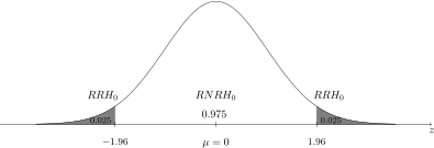
Since the value of the calculated statistic \(Z_c\) \(=\) -2.95 belongs to the rejection region of the hypothesis, then by the binomial test, using the normal approximation, with approximately \(95\%\) confidence, we must reject the null hypothesis that the genes are independent, that is, the halo color and disease resistance genes are linked and, therefore, on the same chromosome. Breeders often want light halos and disease-resistant genotypes. Linkage hinders obtaining such genotypes.
-
9.2.12 The classical formula to determine the sample size is
\(\seteqnumber{0}{9.}{0}\)\begin{align*} n=& \dfrac {Z^2_{\alpha /2}\hat {p}(1-\hat {p})}{e^2}. \end{align*} This formula requires an estimate of \(p\). For this we need a pilot sample, which there is not in this case. An alternative is to use a conservative value of \(n\), in which this expression is maximized with respect to \(\hat {p}\). For this, the previous expression is differentiated with respect to \(\hat {p}\), the result set equal to \(0\) and after solving the equation, we have as solution \(\hat {p}\) \(=\) 0.5. The study of the second derivative proves that this value maximizes the value of \(n\). Thus, the resulting expression is:
\(\seteqnumber{0}{9.}{0}\)\begin{align*} n=& \dfrac {Z^2_{\alpha /2}}{4e^2}. \end{align*} This expression will be used in the present exercise. Thus, with \(95\%\) and margin of error of \(e\) \(=\) 0.05 (do not be confused, reader, there is no relationship of the \(95\%\) confidence or of \(\alpha \) \(=\) \(5\%\) with the value of \(e\) \(=\) \(5\%\), which in this case is equal to \(\alpha \)-mere coincidence). With the confidence value we have \(Z_{\alpha /2}\) \(=\) \(Z_{0.025}\) \(=\) 1.96. Thus,
\(\seteqnumber{0}{9.}{0}\)\begin{align*} n=& \dfrac {1.96^2}{4\times 0.05^2}=384.16\\ =& 385. \quad \textrm {(rounding always upward).} \end{align*} Thus, \(385\) sampling units are necessary to estimate the proportion in this population with \(95\%\) and error upward and downward of \(5\) percentage points. We can also use another more precise formula, such as those presented in the Book.
If we fix \(e\) and \(1-\alpha \) the only way to try to reduce the sample size is to use the first expression, which depends on a pilot sample so that we can estimate \(p\). However, there will only be a reduction in sample size if the sampled binomial population has a parameter \(p\) far from 0.5. Thus, since we do not know the population, for obvious reasons, there is no guarantee that the sample size will be reduced if we use a pilot sample. Note that \(\hat {p}(1-\hat {p})\) is maximum when \(\hat {p}\) \(=\) 0.5, whose maximum value is 0.25. If \(\hat {p}\) moves away from 0.5, then the value of \(\hat {p}(1-\hat {p})\) moves away from 0.25, reducing the value of \(n\) needed. When using the second form, in the worst situation, \(p\) \(=\) 0.5, the \(n\) is determined fairly. If this is not true, \(n\) is overdetermined (sample larger than necessary).
-
9.2.13 We should use the interval for binomial proportions initially, which is given by:
\(\seteqnumber{0}{9.}{0}\)\begin{align} \label {eb9:eq:gex13a} CI_{1-\alpha }(p):& \left [p_I=\dfrac {1}{1+\delta _1},\,\, p_S=\dfrac {1}{1+\delta _2} \right ], \end{align} where
\(\seteqnumber{0}{9.}{1}\)\begin{align*} \delta _1&= \dfrac {(n-s+1)F_{\alpha /2;\nu _1 = 2(n-s+1),\nu _2=2s}}{s} &\textrm { and }&& \delta _2=& \dfrac {n-s}{(s+1) F_{\alpha /2; \nu _1=2(s+1),\nu _2=2(n-s)}}, \end{align*} where \(F_{\alpha /2}\) is the upper quantile of the \(F\) distribution with \(\nu _1\) and \(\nu _2\) degrees of freedom. If \(s = 0\), then \(p_I = 0\) and \(p_S\) must be obtained in (9.1); if \(s = n\), then \(p_S = 1\) and \(p_I\) must be obtained in (9.1). The quantity \(s\) means the number of elements of the random sample that is less than or equal to the sample median \(m_d\).
The ordered sample is:
14 16 16 16 18 19 20 23 24 30 Thus the sample median is \(m_d\) \(=\) 18.5. The value \(s\) is given by \(s\) \(=\) \(5\). Therefore, if we use expression (9.1), we have \(p_I\) \(=\) 0.187086 and \(p_S\) \(=\) 0.812914, using a coefficient of \(95\%\). Finally, the confidence intervals for the median is obtained by
\(\seteqnumber{0}{9.}{1}\)\begin{align*} \left \{\begin{array}{ll} X_I =& (1-g_1)X_{(j)}+ g_1X_{(j+1)} \\ \\ X_S =& (1-g_2)X_{(k)}+ g_2X_{(k+1)} \end {array} \right . \end{align*} where \(j\) \(=\) \(\lfloor np_I \rfloor \), \(g_1\) \(=\) \(np_I\) \(-\) \(j\), \(k\) \(=\) \(\lfloor np_S \rfloor \), \(g_2\) \(=\) \(np_S\) \(-\) \(k\) and \(X_{(0)}\) \(=\) \(X_{(1)}\), if \(j=0\). In this case, we have \(j\) \(=\) \(\lfloor 10\times 0.187086\rfloor \) \(=\) \(1\), \(g_1\) \(=\) 1.87086\(-1\) \(=\) 0.87086, \(k\) \(=\) \(\lfloor 10\times 0.812914 \rfloor \) \(=\) 8, \(g_2\) 8.12914\(-8\) \(=\) 0.12914. Thus,
\(\seteqnumber{0}{9.}{1}\)\begin{align*} X_I =& (1-0.87086)X_{(1)}+ 0.87086X_{(1+1)}\\ =& 0.12914\times 14 + 0.87086\times 16 \\ =& 15.7417. \end{align*} Likewise,
\(\seteqnumber{0}{9.}{1}\)\begin{align*} X_I =& (1-0.12914)X_{(8)}+ 0.12914X_{(8+1)}\\ =& 0.87086\times 23 + 0.12914\times 24 \\ =& 23.1291. \end{align*}
The \(95\)% confidence interval for \(\mu _d\) is [15.74, 23.13]. We also made the confidence interval with bias correction and the result was [16, 23].
-
9.2.14 Let us start by applying the sign test. The hypothesis of interest is
\(\seteqnumber{0}{9.}{1}\)\begin{align*} H_0:\,\, \mu _d=&\mu _{d0}=5.06 &\textrm { versus } && H_0:\,\, \mu _d\ne &5.06. \end{align*} The ordered sample is:
3.51 4.01 5.68 5.84 6.22 6.24 6.29 6.55 7.88 8.04 8.35 Summary of the signs obtained is presented below.
Signs Frequency \(-\) 2 \(0\) 0 \(+\) 9 Thus,
\[n_t = n^+ + n^- =9+2=11=n\]
.
Since \(s = n^+ = 9\) is greater than the expected mean value of positive signs, \(n_t(1- q)\) \(=\) \(11\times 0.5\) \(=\) 5.5, the \(p\)-value, with \(q\) \(=\) 0.5, is
\(\seteqnumber{0}{9.}{1}\)\begin{align*} \textrm {$p$-value}=& 2P(S\ge s)=2P(S\ge 9)\\ =& 2\sum _{i=s}^{n_t} \binom {n_t}{i}(1-q)^iq^{n_t-i} = 2 \left (\dfrac {1}{2}\right )^{11} \sum _{i=9}^{11} \binom {11}{i}\\ =& \left (\dfrac {1}{2}\right )^{10} \left (55 + 11 +1\right )=\dfrac {67}{1024}=0.06542969. \end{align*}
The \(F\) distribution can be used, which has an advantage for large values of \(n_t\), whose calculated value, replacing \(s\) by \(s-1\) \(=\) \(8\), is
\(\seteqnumber{0}{9.}{1}\)\begin{align*} F_c=& \dfrac {s+1}{n_t-s}\times \dfrac {q}{1-q}\\ =& \dfrac {8+1}{11-8}\times \dfrac {0.5}{1-0.5}=3. \end{align*} with \(\nu _1=2(11-8)=6\) and \(\nu _2=2(8+1) = 18\) degrees of freedom.
The following \(p\)-value found is
\(\seteqnumber{0}{9.}{1}\)\begin{align*} 2(1-P(F < 3;\nu _1=6,\nu _2=18)) =& 2(1-0.9672852) = 0.06542969. \end{align*}
Both procedures provide the same \(p\)-value (0.06542969), because they are equivalent procedures. Since the \(p\)-value is greater than \(5\%\) (nominal value adopted) the null hypothesis should not be rejected at the nominal significance value of \(5\%\), that is, the median fat content of the milk of the sampled breed can be considered equal to \(3\%\). The reader is invited to consider \(S\) as being the number of values below \(m_{d0}\), that is, whose observed value is \(n^-\) and with \(p\) \(=\) \(q\). After this, reproduce the results of this example and verify that they are essentially equal.
In the second stage, let us apply the signed rank test. The null and alternative hypotheses are the same as presented in the first stage. We must initially compute the signed ranks, from the ordered sample previously presented. In the following table the ten observations are presented with the differences \(d_i\)’s, the ranks obtained considering the absolute values of the \(d_i\)’s and the respective associated signs, in parentheses.
Observation \((x_i)\) \(d_i=x_i-\mu _{d0}\) (sign) rank 3.51 -1.55 \((-)\) 8 4.01 -1.05 \((-)\) 3 5.68 0.62 \((+)\) 1 5.84 0.78 \((+)\) 2 6.22 1.16 \((+)\) 4 6.24 1.18 \((+)\) 5 6.29 1.23 \((+)\) 6 6.55 1.49 \((+)\) 7 7.88 2.82 \((+)\) 9 8.04 2.98 \((+)\) 10 8.35 3.29 \((+)\) 11 The number of non-null differences is \(n_t\) \(=\) \(n\) \(=\) \(11\) and the value of \(T^+\) is \(t^+\) \(=\) \(1 + 2 + 4+5+6+7+9+10+11\) \(=\) \(55\). Consulting Table A.10 we obtain the critical limits for the test, considering \(\alpha \) equal to \(5\%\) and \(n_t=11\). The tabulated critical limit is \(T^+_{0.975}=10\). The upper critical limit is obtained by
\(\seteqnumber{0}{9.}{1}\)\begin{align*} T^+_{\alpha /2}=& \dfrac {n_t\left (n_t+1\right )}{2}-T^+_{1-\alpha /2} = \dfrac {11\times 12}{2}-8=58. \end{align*}
Since \(t^+ = 55\) is between the two critical limits, then it belongs to the non-rejection region of hypothesis \(H_0\) and, therefore, there is no reason to suspect that the median amount of nitrate in Minas Gerais is different from the median of the United States, considering the nominal significance of \(5\)% . The result agrees with the value obtained by the sign test (without ranks).
Finally, let us present the normal approximation (without continuity correction) of this last test. The mean and variance of \(T^+\), since there were no ties, are
\(\seteqnumber{0}{9.}{1}\)\begin{align*} \mu _{T^+}=& \dfrac {n_t\left (n_t+1\right )}{4}=\dfrac {11\times 12}{4}=33 \\ \textrm { and }&\\ \sigma ^2_{T^+}=& \dfrac {n_t\left (n_t+1\right ) \left (2n_t+1\right )}{24}=\dfrac {11\times 12\times 23}{24} = 126.5. \end{align*}
The value of the statistic, with continuity correction, considering \(t^+ = 55\), is
\(\seteqnumber{0}{9.}{1}\)\begin{align*} Z_c=& \dfrac {55-33}{\sqrt {126.5}}=1.956. \end{align*}
Since \(Z_c\), without continuity correction, is between the normal critical limits \(-Z_{0.025}\) \(=\) \(-\)1.96 and \(Z_{0.025}\) \(=\) 1.96, the null hypothesis \(H_0\) should not be rejected at the nominal significance value of \(5\%\). The \(p\)-value is 0.0505, reinforcing this result. Note that by a very small margin, the normal approximation did not provide a result different from the exact method. This fact highlights the importance of having exact methods.
-
9.2.15 Considering that the distribution of the population is normal, knowing that \(s^2\) \(=\) 1.6, \(n=37\), \(\chi ^2_{0.975;\nu =36}\) \(=\) 21.3359 and \(\chi ^2_{0.025;36}\) \(=\) 54.4373, we have
\(\seteqnumber{0}{9.}{1}\)\begin{align*} CI_{1-\alpha }\left (\sigma ^2\right ):&\,\,\left [\dfrac {(n-1)S^2}{\chi ^2_{\alpha /2;\nu }}, \,\, \dfrac {(n-1) S^2}{\chi ^2_{1-\alpha /2;\nu }}\right ]\\ :& \left [\dfrac {36\times 1.6}{54.4373}, \,\, \dfrac {36\times 1.6}{21.3359}\right ]\\ :&\,\,[1.0581,\,\,2.6997]. \end{align*}
With \(95\%\) confidence, the true population variance is a value contained in the interval [1.0581, 2.6997]. Since the value of the variance of the single hybrid is 0.6, we can conclude, with \(95\%\) confidence, that the variance of the triple hybrid is greater than that of the single hybrid. This result is expected, since the variability of a single hybrid is merely from environmental factors, while the variance of the triple hybrid contains a genetic source of variability, in addition to the environmental source.
-
9.2.16 To perform the test on the variance, we will adopt the following procedures. We formulate the null and alternative hypotheses by:
\(\seteqnumber{0}{9.}{1}\)\begin{align*} H_0:\, \sigma ^2\le & 0.6 &\textrm { vs }&& H_1:\, \sigma ^2 > & 0.6. \end{align*}
The test statistic is calculated using:
\(\seteqnumber{0}{9.}{1}\)\begin{align*} \chi ^2_c=& \dfrac {(n-1)S^2}{\sigma ^2_0}=\dfrac {36\times 1.6}{0.6}=96. \end{align*}
The critical region (of rejection of the hypothesis) for the test is given by:
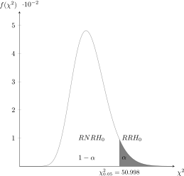
as \(\chi ^2_c=96\) is located in the rejection region of the null hypothesis, we must reject hypothesis \(H_0\), considering the chi-square test with \(95\%\) confidence. Thus, the hypothesis that the population variance is equal to or less than 0.6 \(t^2\)/ha must be rejected and, therefore, the triple hybrid is more variable than the single hybrid. This is a good example to show how tests often corroborate our theories. In this case, we know that the variation of the single hybrid has two origins, the environmental and genetic variabilities. The single hybrid has present only the environmental source of variation and, therefore, should present less variability than the triple hybrid.
-
9.2.17 The McKay modified interval, as acclaimed by Vangel (1996) as the best approximation, is
\(\seteqnumber{0}{9.}{1}\)\begin{align*} CI_{1-\alpha }(\kappa ): & \left [\kappa _I,\,\, \kappa _S \right ]. \end{align*} where
\(\seteqnumber{0}{9.}{1}\)\begin{align*} \kappa _I =& \dfrac {K}{\sqrt {\left (\dfrac {\chi ^2_{\alpha /2;\nu }+2}{\nu +1}- 1 \right ) K^2+ \dfrac {\chi ^2_{\alpha /2;\nu }}{\nu }}} \end{align*} and
\(\seteqnumber{0}{9.}{1}\)\begin{align*} \kappa _S =& \dfrac {K}{\sqrt {\left (\dfrac {\chi ^2_{1-\alpha /2;\nu }+2}{\nu +1}- 1 \right )K^2+ \dfrac {\chi ^2_{1-\alpha /2;\nu }}{\nu }}}, \end{align*} where \(\nu \) \(=\) \(n-1\).
In the present case, we have \(K\) \(=\) 0.32 and \(\bar {X}\) \(=\) 0.0307, with \(n=100\). Thus, \(\chi ^2_{\alpha /2;\nu }\) \(=\) \(\chi ^2_{0.025;\nu =99}\) \(=\) 128.422 and \(\chi ^2_{1-\alpha /2;\nu }\) \(=\) \(\chi ^2_{0.975;\nu =99}\) \(=\) 73.361. Thus,
\(\seteqnumber{0}{9.}{1}\)\begin{align*} \kappa _I =& \dfrac {0.32}{\sqrt {\left (\dfrac {128.422+2}{99+1}- 1 \right ) 0.32^2+ \dfrac {128.422}{99}}}=\dfrac {0.32}{1.152538}\\ =& 0.2776 \end{align*} and
\(\seteqnumber{0}{9.}{1}\)\begin{align*} \kappa _S =& \dfrac {0.32}{\sqrt {\left (\dfrac {73.361+2}{99+1}- 1 \right ) 0.32^2+ \dfrac {73.361}{99}}}=\dfrac {0.32}{0.8460442}\\ =& 0.3782. \end{align*} Finally, the \(95\%\) interval for the population coefficient of variation \(\kappa \) is
\(\seteqnumber{0}{9.}{1}\)\begin{align*} CI_{0.95}(\kappa ): & \left [0.2776,\,\, 0.3782 \right ]. \end{align*}
-
9.2.18 In a sample of size \(n=10\) the value of the \(CV\) was 0.1502. The hypotheses of interest, null and alternative, are
\(\seteqnumber{0}{9.}{1}\)\begin{align*} H_0:\, \kappa =& 0.05 &\textrm { vs }&& H_1:\, \kappa \ne & 0.05. \end{align*}
The test statistic is calculated using:
\(\seteqnumber{0}{9.}{1}\)\begin{align*} \chi ^2_c=& \dfrac {\nu K^2 \left [\nu +1+(\nu +1)\kappa _0^2\right ]}{\kappa _0^2 \left (\nu +1 + \nu K^2\right )}, \end{align*} formulated by McKay (1932), modified by Vangel (1996). An important observation must be made, because in the current edition of the Book, the part \(\nu +1+(\nu +1)\kappa _0^2\) of the numerator of the test statistic expression has an error, because instead of \(\nu +1+(\nu +1)\kappa _0^2\) it is incorrectly presented as \(\nu +1+(\nu -1)\kappa _0^2\). Thus,
\(\seteqnumber{0}{9.}{1}\)\begin{align*} \chi ^2_c=& \dfrac {9\times 0.1502^2 \left (9+1+10\times 0.05^2\right )}{0.05^2 \left (9+1 + 9\times 0.1502^2\right )}\\ =& 79.799. \end{align*}
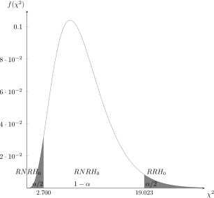
The critical region (of rejection of the hypothesis) for the test is given by: \(\{\chi ^2\le \) 2.700\(\}\cup \{\chi ^2\ge \) 19.023\(\}\). Since \(\chi ^2_c\) \(=\) 79.799 belongs to the rejection region of \(H_0\), we must reject the null hypothesis that the coefficient of variation of this species is not different from that of the reference clone, presenting in fact higher relative variability than the clone in question, by the chi-square test of McKay (1932) with \(95\%\) confidence. See the illustrative graph below.