Basic Statistics
2.2 Solutions
-
2.2.1 Frequency distribution:
-
a) The different criteria differ only in the number of classes used. Thus, we will use only the empirical criterion, Table 2.9, in which the number of classes \(k\) is given by
\(\seteqnumber{0}{2.}{0}\)\begin{align*} k =&\left \{\begin{array}{ll} \sqrt {n} & n\le 100 \quad (\textrm {nearest integer}) \\ 5\log _{10}(n) & n > 100 \quad (\textrm {nearest integer}), \end {array} \right . \end{align*} which results in \(k\) \(=\) \(\sqrt {n}\) \(=\) \(\sqrt {50}\) \(=\) \(7\) classes. The remaining cases are left to the reader to reproduce.
The next step is to determine the total range, given by:
\[ A=X_{(n)}-X_{(1)}=25.52-1.52=24g. \]
Then we compute the class width and the lower limit of the first class by:
\(\seteqnumber{0}{2.}{0}\)\begin{align*} c=& \dfrac {A}{k-1}= \dfrac {24}{6}=4\\ LI_{1} =& X_{(1)}-\dfrac {c}{2}=1.52-2=-0.48. \end{align*} Thus, the resulting frequency distribution is:
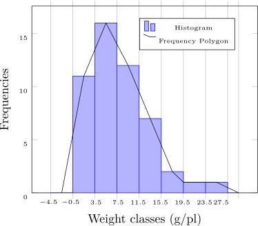
Yield classes \(\bar {X}_i\) \(F_i\) \(Fr_i\) \(Fp_i\)(%) \(-0.48\vdash \,\,3.52\) 1.52 11 0.22 22 \(\,\,\,\, 3.52\vdash 7.52\) 5.52 16 0.32 32 \(\,\,\,\, 7.52\vdash 11.52\) 9.52 12 0.24 24 \(\,11.52\vdash 15.52\) 13.52 7 0.14 14 \(\,15.52\vdash 19.52\) 17.52 2 0.04 4 \(\,19.52\vdash 23.52\) 21.52 1 0.02 2 \(\,23.52\vdash 27.52\) 25.52 1 0.02 2 The remaining criteria follow the same pattern and will not be shown, possibly differing only in the number of classes. If this occurs, obviously the other quantities change. It is left to the reader to verify such facts.
-
b) The histogram and the frequency polygon were plotted on the same graph, yielding:
-
c) The cumulative frequency distribution table for this case is:
Limits \((x_i)\) \(FC(X<x_i)\) \(FC(X\ge x_i)\) \(\,\, -0.48\) 0 50 \(\,\,\, 3.52\) 11 39 \(\,\,\, 7,52\) 27 23 \(11.52\) 39 11 \(15.52\) 46 4 \(19.52\) 48 2 \(23.52\) 49 1 \(27.52\) 50 0 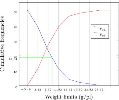
-
d) Percentage of plants with yield greater than \(9\):
-
i) Using direct counting in the original data, we see that \(18\) values exceed the value \(9\). Thus, with a simple rule of three we extrapolate the estimate to the general case, that is, we say that \(36\%\) of the plants yield more than \(9\) g.
-
ii) Using the ogive: in the previous figure, we plotted the line corresponding to the value \(9\) and found the ogive \(F_{c\downarrow }\). The graphical reading resulted in the approximate value of 18.64. This value corresponds to 37.28% of the plants with yield greater than \(9\) g.
-
iii) In the frequency distribution we have that the value \(9\) is in the third class. The remaining classes, higher than the third, have values that are known to be greater than \(9\) and total \(11\) plants. It remains to discover, by geometric interpolation, how many of the \(12\) plants are greater than \(9\) in the third class. We use the rule of three and assume that the distribution within the class is uniform. Thus,
\(\seteqnumber{0}{2.}{0}\)\begin{align*} 11.52-7.52=4.00 \longrightarrow & F_3=12\\ 11.52-9.00=2.52 \longrightarrow & x, \end{align*} resulting in \(x\) \(=\) 7.56 plants exceed \(9\) g of yield. Thus, the total is 7.56 \(+\) 11 \(=\) 18.56. This value corresponds to 37.12% of the plants with yield greater than \(9\) g.
The three answers, from the three different methods, were very close to each other, as expected. The “exact” value (best estimate of the population proportion) was \(36\%\) and the errors upward were 1.28 and 1.12 percentage points. In relative terms these errors were 3.56% and 3.11%, respectively, for geometric interpolation and algebraic interpolation.
-
-
e) From the observation of the frequency distribution we can say that the distribution is right-skewed, although the degree of skewness is not very intense. This phenomenon is compatible with segregation in quantitative characters with dominance (quantitative inheritance in the presence of dominance).
-
f) The stem-and-leaf plot can be made in R with the command stem(prod), where prod is the vector of original data. The result is given by:
 0 | 5
 2 | 2489012455899
 4 | 4682
 6 | 025677813
 8 | 0248022246
10 | 19
12 | 015899
14 | 2
16 | 6
18 | 4
20 |
22 | 1
24 | 5
A more modern version is the BoxPlot, made with the command boxplot(prod) in R, presented below:
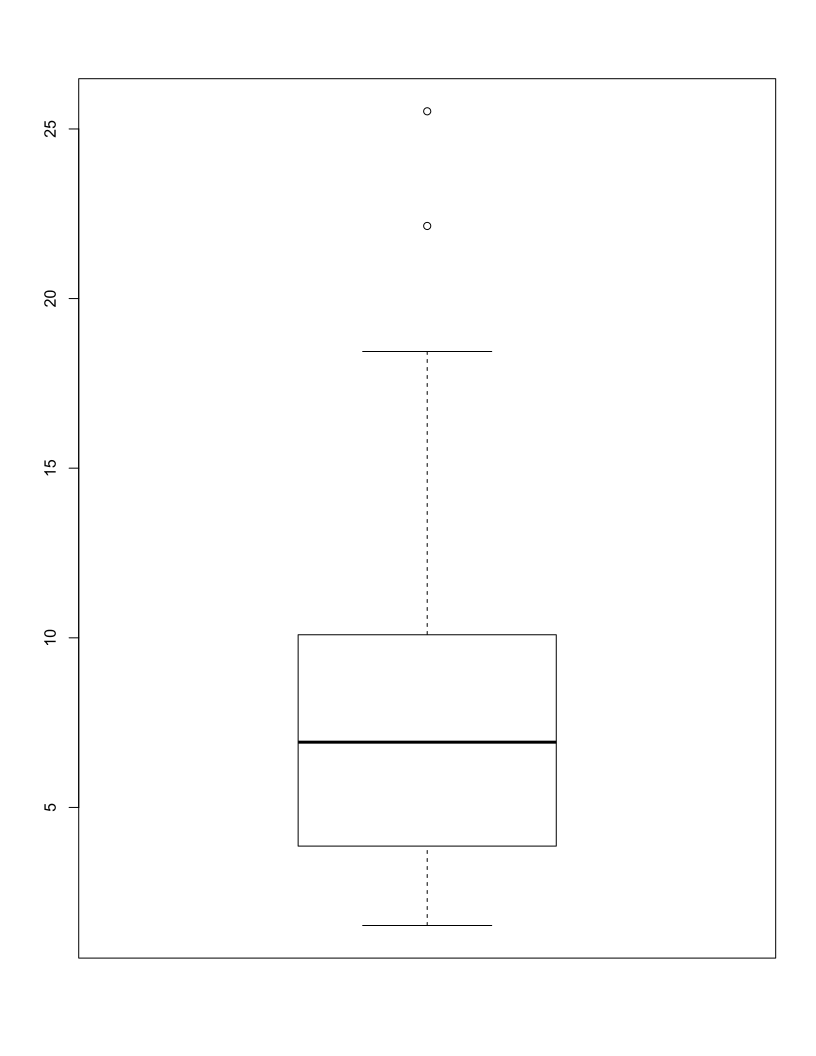
In this graph, we can observe the minimum, excluding potential outliers, the maximum, also excluding outliers, the median, the first quartile (\(25\%\) percentile), and the third quartile (\(75\%\) percentile).
-
g) Determine the yield above which \(50\%\) of the plants (\(25\) plants) are:
-
i) By direct observation of the ordered data, given by:
1.52 2.23 2.39 2.81 2.85 3.01 3.10 3.19 3.38 3.49 3.50 3.76 3.86
3.90 4.43 4.64 4.80 5.15 6.02 6.20 6.53 6.61 6.71 6.73 6.78 7.07
7.33 7.97 8.23 8.40 8.75 8.99 9.15 9.19 9.20 9.40 9.60 10.09 10.86
12.95 13.12 13.46 13.84 13.86 13.94 14.20 16.56 18.44 22.14 25.52
we can observe that the desired value is between 6.78 and 7.07. Any value between these two numbers is a potential value for our answer. We can agree to take the average of the two. Thus, the answer is 6.925 g.
-
ii) A second alternative is to use the graphical method, through the ogives. We select the value \(25\) on the abscissa and find the cumulative frequency curve \(F_{c\uparrow }\). The corresponding value on the abscissa is the desired value, as illustrated in the figure below:
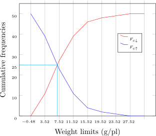
This value corresponds to the value 7.03 g on the abscissa. Thus, \(50\%\) of the plants exceed 7.03 g, by this method.
-
iii) By algebraic interpolation in the frequency distribution, we have that above 7.52 g there are \(23\) plants and above 3.52, \(39\) plants. Thus, the desired value lies in the second class and can be obtained by interpolation. Since above 7.52 we have \(23\) plants, above the desired value in the second class there are \(25\), between the desired value and the upper limit 7.52 g another \(2\) plants are needed to complete the \(25\) required. Thus:
\(\seteqnumber{0}{2.}{0}\)\begin{align*} 4 \longrightarrow & 16 \\ x \longrightarrow & 2, \end{align*} resulting in \(x\) \(=\) 0.50 g. The desired value is therefore 7.52\(-\)0.50 \(=\) 7.02 g. Thus, \(50\%\) of the plants exceed 7.02 g, by this method.
The three methods again led to very similar results, and any of them can be chosen to estimate such upper quantiles or to estimate lower quantiles. This will depend only on what type of information is available to the reader when estimating such quantities.
-
-
h) To obtain the percentage of values with yield below 3.5 g we will use only algebraic interpolation in the frequency distribution. The other two methods can be applied as in the previous cases. The value of 3.5 lies in the first class. Thus,
\(\seteqnumber{0}{2.}{0}\)\begin{align*} 4 \longrightarrow & 11 \\ 3.5-(-0.48)=3.98 \longrightarrow & x, \end{align*} resulting in “10.945 plants”. Considering that \(100\%\) correspond to \(50\) plants, then 10.945 correspond to 21.89%. Therefore, 21.89% of the plants yield less than 3.50 g.
-
i) Again we will use only algebraic interpolation in the frequency distribution. For the value that leaves below it \(25\%\) of the plants (12.5 plants), we have that it lies in class \(2\). In class \(1\) we have \(11\) plants. Thus, 1.5 more plants are needed to complete the 12.5 plants. Therefore, of the \(16\) plants in the class, we need to find the value that leaves 1.5 of them below it. Thus,
\(\seteqnumber{0}{2.}{0}\)\begin{align*} 4 \longrightarrow & 16 \\ x \longrightarrow & 1.5, \end{align*} resulting in \(x\) \(=\) 0.375. The desired value is 3.52\(+\)0.375 \(=\) 3.895. Thus, \(25\%\) of the plants are below 3.895 g.
For the value that leaves \(25\%\) of the plants (12.5 plants) above it, we verify that above 11.52 g we have \(11\) plants. 1.5 plants are needed in class \(3\). Thus,
\(\seteqnumber{0}{2.}{0}\)\begin{align*} 4 \longrightarrow & 12 \\ x \longrightarrow & 1.5, \end{align*} resulting in \(x\) \(=\) 0.50. The desired value is 11.52\(-\)0.50 \(=\) 11.02. Thus, \(25\%\) of the plants are above 11.02 g.
-
-
2.2.2 The variable number of galls per plant was analyzed as follows:
-
a) The graph of the occurrence of galls is given by:
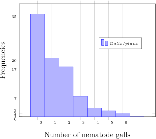
It is verified that the distribution is right-skewed. The variable of Exercise 1 is quantitative continuous and the variable of the current exercise is quantitative discrete.
-
b) The cumulative frequency distribution table for this case is:
\(x_i\) \(FC(X\le x_i)\) \(FC(X > x_i)\) \(FC_r(X\le x_i)\) \(FC_r(X > x_i)\) \(-1\) 0 85 0.00 1,00 \(0\) 35 50 0.41 0.59 \(1\) 55 30 0.65 0.35 \(2\) 72 13 0.85 0.15 \(3\) 79 6 0.93 0.07 \(4\) 82 3 0.96 0.04 \(5\) 84 1 0.99 0.01 \(6\) 85 0 1.00 0.00 \(7\) 85 0 1.00 0.00 -
c) It is potentially possible to find such a plant with more than \(6\) galls, even in an area of low nematode incidence like this one. For this, it is necessary to increase the sample size, since plants with such infestation, as indicated by the data and the previous graph, are at low frequency in the sampled population. Thus, these elements at low frequency in the population would have higher chances of being sampled in large samples.
-
-
2.2.3 Let the samples of size \(n=5\) be given by:
\(\seteqnumber{0}{2.}{0}\)\begin{align*} X=&\left \{2, 4, 4, 3, 2\right \}\\ Y=&\left \{1, 2, 3, 6, 7\right \}, \end{align*} then:
i) \(\displaystyle \sum _{j=1}^4 x_j = \) \(x_1+x_2+x_3+x_4=\) \(2+4+4+3=13\);
ii) \(\displaystyle \sum _{j=1}^5 4x_j^2 =2 \sum _{j=1}^5 x_j^2=\) \(4\times (2^2+4^2+\ldots +2^2)=2\times 49=196\);
iii) \(\displaystyle \sum _{j=1}^5 (3x_j+2y_j)=3\sum _{j=1}^5 x_j+ 2\sum _{j=1}^5 y_j=\) \(3\times 15 + 2\times 19=83\);
iv) \(\displaystyle \sum _{j=1}^5 y_j =\) \(y_1+\ldots +y_5=\) \(1+2+\ldots +7=19\);
v) \(\displaystyle \sum _{j=1}^5 x_j y_j =\) \(2\times 1+ 4\times 2+ \ldots + 2\times 7=\) \(2+8+\ldots +14=54\); and
vi) \(\displaystyle \sum _{j=2}^4 x_jy_j + \sum _{j=1}^5 y_j^2=\) \(40+(1^2+2^2+\ldots +7^2)=40+99=139.\)
Show numerically and algebraically that the sums of deviations from the arithmetic mean are zero, whatever the sample, using the set \(X\) given above for the numerical case:
a) Numerically
The mean is:
\(\seteqnumber{0}{2.}{0}\)\begin{align*} \bar {X} =& \dfrac {\displaystyle \sum _{j=1}^{n} X_j}{n}=\dfrac {13+2}{5}=3 \end{align*}
\(\displaystyle \sum _{j=1}^n(X_j-\bar {X})=(2-3)+(4-3)+\ldots +(2-3)=-1+1+1+0-1=0\);
b) algebraically
\(\seteqnumber{0}{2.}{0}\)\begin{align*} \sum _{j=1}^n(X_j-\bar {X})=& \sum _{j=1}^nX_j-\sum _{j=1}^n\bar {X}=\sum _{j=1}^nX_j-n\bar {X}\\ =& \sum _{j=1}^nX_j-\dfrac {\cancel {n} \displaystyle \sum _{j=1}^n X_j}{\cancel {n}}=\sum _{j=1}^nX_j-\sum _{j=1}^nX_j=0,\quad \textrm { Q.E.D.} \end{align*}
Finally, for the data from the two-way table of grass yields, the following sums
\(i. \displaystyle \sum _{i=1}^4\sum _{j=1}^3 X_{ij}^2 = (4.6^2+\cdots +5.5^2+\cdots +6.0^2+\cdots +6.8^2\) \(=\) \(76.41+92.46+101.64+120.68\) \(=\) \(391.19\)
\(ii. \displaystyle \sum _{i=1}^4 X_{ij}^2 \quad j=1,2,3\)
We have:
\(\seteqnumber{0}{2.}{0}\)\begin{align*} \sum _{i=1}^4 X_{i1}^2 =& 4.6^2+\cdots +6.0^2=109.20 \quad j=1\\ \sum _{i=1}^4 X_{i2}^2 =& 5.0^2+\cdots +6.2^2=127.33 \quad j=2\\ \sum _{i=1}^4 X_{i3}^2 =& 5.5^2+\cdots +6.8^2=154.66 \quad j=3 \end{align*}
\(iii. \displaystyle \sum _{j=1}^3 X_{ij}^2 \quad i=1,2,3,4\)
We have:
\(\seteqnumber{0}{2.}{0}\)\begin{align*} \sum _{j=1}^3 X_{1j}^2 =& 4.6^2+5.0^2+5.5^2=76.41 \quad i=1\\ \sum _{j=1}^3 X_{2j}^2 =& 5.0^2+5.5^2+6.1^2=92.46 \quad i=2\\ \sum _{j=1}^3 X_{3j}^2 =& 5.2^2+5.8^2+6.4^2=101.64 \quad i=3\\ \sum _{j=1}^3 X_{4j}^2 =& 6.0^2+6.2^2+6.8^2=120.68 \quad i=4 \end{align*}
-
2.2.4 Milk yield data:
-
a) The mean and the midrange are:
\(\seteqnumber{0}{2.}{0}\)\begin{align*} \bar {X} =& \dfrac {\displaystyle \sum _{j=1}^{n} X_j }{n}=\dfrac {299.7}{30} =9.99 \\ \bar {X}_{0.50} =& \dfrac {X_{(1)}+X_{(n)}}{2}=\dfrac {8.13+12.14}{2}=10.135. \end{align*}
-
b) The trimmed mean:
\(\seteqnumber{0}{2.}{0}\)\begin{align*} \bar {X}_A =& \dfrac {\displaystyle \sum _{j=3}^{n-2} X_j }{n}=\dfrac {8.6+\cdots +11.46}{26} =\dfrac {259.15}{26}=9.9673. \end{align*}
In this case there is no evidence of any outlier or discrepant data. The frequency distribution (not shown) is reasonably symmetric, and therefore there is no need to use this estimator. Moreover, the estimates of both estimators are reasonably close, corroborating the argument that the trimmed mean is unnecessary.
-
c) The median, since \(n\) is even, must be computed by:
\(\seteqnumber{0}{2.}{0}\)\begin{align*} m_d =& \dfrac {X_{\left (\frac {n}{2}\right )} +X_{\left (\frac {n+2}{2}\right )}}{2} = \dfrac {X_{(15)} + X_{(16)}}{2} = 10.055 l. \end{align*}
From the order statistics, since the data are quantitative continuous and \(P(X=x)=0\) \(\forall x\in \mathbb {R}\), it is not possible to estimate the mode by looking at the value that repeats most or is most frequent. In the next exercise we will present an estimate of the population mode.
-
d) The \(5\%\) and \(95\%\) percentiles by method \(1\) of the weighted mean (we used Sisvar) are:
\(\seteqnumber{0}{2.}{0}\)\begin{align*} X_{0.05}=& 8.18 &\textrm { and }&& X_{0.95}=&11.76 l. \end{align*} By method \(2\) (nearest observation) they are:
\(\seteqnumber{0}{2.}{0}\)\begin{align*} X_{0.05}=& 8.23 &\textrm { and }&& X_{0.95}=&11.46 l. \end{align*} By method \(3\) (empirical distribution) they are:
\(\seteqnumber{0}{2.}{0}\)\begin{align*} X_{0.05}=& 8.23 &\textrm { and }&& X_{0.95}=&12.05 l. \end{align*} By method \(4\) (weighted mean) they are:
\(\seteqnumber{0}{2.}{0}\)\begin{align*} X_{0.05}=& 8.185 &\textrm { and }&& X_{0.95}=&12.0905 l. \end{align*} By method \(5\) (empirical distribution with weighting) they are:
\(\seteqnumber{0}{2.}{0}\)\begin{align*} X_{0.05}=& 8.23 &\textrm { and }&& X_{0.95}=&12.05 l. \end{align*}
-
e) Using the property of the arithmetic mean, considering the income represented by \(Y\) \(=\) \(k X\), where \(k\) \(=\) 0.27, we have
\(\seteqnumber{0}{2.}{0}\)\begin{align*} \bar {Y} =& k\bar {X} =0.27\times 9.99=2.70, \end{align*} which corresponds to the average income per liter of milk (price in reais at the time).
-
f) The harmonic and geometric means are:
\(\seteqnumber{0}{2.}{0}\)\begin{align*} \bar {X}_{H} =& \dfrac {1}{\dfrac {1}{n}\displaystyle \sum _{i=1}^n{\dfrac {1}{X_i}}} = \dfrac {1}{\dfrac {1}{30}\displaystyle \sum _{i=1}^n{\dfrac {1}{8.13}+\cdots +\cfrac {1}{12.14}}}=\dfrac {1}{\dfrac {3.031835}{30}} = 9.8950\\ \bar {X}_{G} =& \sqrt [n]{\prod _{i=1}^nX_i} = \sqrt [30]{8.409706\times 10^{29}}=9.9424. \end{align*}
The relationship among the mean, geometric mean, and harmonic mean, given by \(\bar {X}_H \le \bar {X}_G \le \bar {X}\) was verified, which in this case corresponds to the following relationship: 9.90\(<\)9,94\(<\)9.99. Equality occurs only if all sample values are equal.
-
-
2.2.5 Calculate the measures of location in the frequency distribution: To group the data one must obtain:
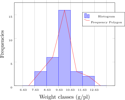
The number of classes is given by \(k=\sqrt {n}=\sqrt {30} \approx 5\) and the total range by \(A=x_{(30)}-x_{(1)}=\)12.14\(-\)8.13=4.01. Thus, the class width is given by \(c=A/(k-1)=\)4.01/4\(\approx \) 1.00 and the lower limit of the first class by \(LI_1 = x_{(1)}-c/2=\)8.13\(-\)1.00/2=7.63. The remaining class limits are obtained by adding \(c=\)1.00 to the previously obtained limits. The frequency distribution obtained in this way is:
Weight classes \(\bar {X}_i\) \(F_i\) \(Fr_i\) \(Fp_i\)(%) 7.63 \(\vdash \) 8.63 8.13 3 0.10 10.00 8.63 \(\vdash \) 9.63 9.13 6 0.20 20.00 9.63 \(\vdash \) 10.63 10.13 16 0.53 53.33 10.63 \(\vdash \) 11.63 11.13 3 0.10 10.00 11.63 \(\vdash \) 12.63 12.13 2 0.07 6.67 -
i) The arithmetic mean is given by:
\(\seteqnumber{0}{2.}{0}\)\begin{align*} \bar {X}=& \dfrac {\displaystyle \sum _{i=1}^k F_i \bar {X}_i}{n}=\dfrac {8.13\times 3+ 9.13\times 9+ 10.13\times 16+ 11.13\times 3+ 12.13\times 2}{30}\\ =& \dfrac {298.9}{30} = 9.9633 \end{align*}
The difference found for the mean of the ungrouped data can be attributed to grouping. Every way of representing the data in a more simplified (summarized) manner leads to some kind of loss of precision. For example, the loss of precision in this case is due to the basic tabular hypothesis, in which the midpoints of each class are used to represent all values in it. What should be clear, however, is that despite being less precise, the estimate obtained from the grouped data is a “reliable estimate” in a certain sense of the population mean, as much as the estimate from the original data. The loss of precision is generally small and can be considered negligible.
The median is obtained as follows. The median class is the one containing position number \(n/2=30/2=15\). Therefore, the median class is the third, since the cumulative frequencies of the first two classes sum to only \(9\), which is less than \(15\). Thus,
\(\seteqnumber{0}{2.}{0}\)\begin{align*} m_d =& LI_{m_d}+\dfrac {\frac {n}{2}-F_A}{F_{m_d}}c_{m_d}=9.63+\dfrac {15-9}{16}\times 1.00\\ =& 10.0050 \end{align*}
The same observation made for the difference in the mean estimates applies to the median.
To obtain the mode, it is necessary to determine the class with the highest frequency, that is, the modal class. The modal class in this exercise is the third. The difference between the frequencies of the modal class and the previous class is \(\Delta _1=16-6=10\) and the difference between the frequencies of the modal class and the following class is \(\Delta _2=16-3=13\). Thus, we have
\(\seteqnumber{0}{2.}{0}\)\begin{align*} m_o=& LI_{m_o} + \dfrac {\Delta _1}{\Delta _1+\Delta _2} c_{m_o}=9.63+\dfrac {10}{10+13}\times 1.00\\ =& 10.0648. \end{align*}
The three measures, mean, median, and mode, are very close, and this is an indication that the data distribution should be approximately symmetric. The mode cannot be calculated from the original data when the data are quantitative continuous, that is, in continuous random variables where \(P(X=x)=0\) \(\forall x\in \mathbb {R}\).
-
ii) The geometric mean is
\(\seteqnumber{0}{2.}{0}\)\begin{align*} \bar {X}_{G} =& \exp \left (\dfrac {\displaystyle \sum _{i=1}^k F_i \ln (\bar {X}_i)}{n} \right )=\exp \left (\dfrac {6.2867+\cdots +4.9914}{30} \right )\\ =& \exp \left (\dfrac {68.82439}{30}\right )=9.915969. \end{align*} The harmonic mean is:
\(\seteqnumber{0}{2.}{0}\)\begin{align*} \bar {X}_{H} =& \dfrac {1}{\dfrac {1}{n}\displaystyle \sum _{i=1}^k{\dfrac {F_i}{\bar {X}_i}}}=\dfrac {1}{\dfrac {0.3690037+\cdots +0.1648805}{30}}\\ =& \dfrac {1}{0.1013356}=9.868204. \end{align*}
The values of the harmonic and geometric means in the frequency distribution differed only in the second decimal place relative to the same values obtained from the original data. Summarizing the data generally makes them less informative and the estimates in this format less precise. However, in most cases, the loss of precision is not significant.
The quadratic mean is:
\(\seteqnumber{0}{2.}{0}\)\begin{align*} \bar {X}_{MQ} &= \sqrt {\dfrac {\displaystyle \sum _{i=1}^k F_i \bar {X}_i^2}{n}} = \sqrt {\dfrac {198.2907+\cdots +294.2738}{30}} = \sqrt {100.2069}\\ =& 10.01034. \end{align*}
-
iii) The comparisons, when possible, were made in the answers given above. The main reason for the difference is that when summarizing a data set and trying to obtain the same information, there will be a loss of precision as a result.
-
iv) The histogram and frequency polygon are presented below:
-
v) the distribution is approximately symmetric, with a small right skewness. Thus, the mean is the most appropriate measure of location, by virtue of its optimal properties and because there is no pronounced skewness, a condition that harms this estimator relative to the median or mode.
-
vi) Using the information provided in the exercise, we can estimate the total milk yield of the municipality as follows. Each lactating cow produces on average 9.9633 kg and there are on average 8.075 lactating cows per producer and a total of \(7309\) producers, therefore
\(\seteqnumber{0}{2.}{0}\)\begin{align*} \textrm {Total } =& 9.9633\times 8.075\times 7309\\ =& 588035.7 \textrm { kg/day} \end{align*}
-
-
2.2.6 The arithmetic mean, with \(k\) being the number of categories, \(7\) in this case, is:
\(\seteqnumber{0}{2.}{0}\)\begin{align*} \bar {X} =& \dfrac {\displaystyle \sum _{i=1}^{k} x_i F_i}{n}= \dfrac {0\times 35+\cdots +6\times 1}{85}=\dfrac {103}{85}\\ =& 1.2118. \end{align*} The mode is the most frequent value, that is, \(m_o\) \(=\) \(0\), and the median, since \(n=85\) is odd, is given by
\(\seteqnumber{0}{2.}{0}\)\begin{align*} m_d =& x_{((n+1)/2)}=x_{(43)}=1. \end{align*}
The distribution is right-skewed; therefore, the mean is not a good measure to represent these data, since it is influenced by extreme values. Thus, either the median or the mode can be used for this purpose.
-
2.2.7 Calving interval data.
-
a) The range is:
\(\seteqnumber{0}{2.}{0}\)\begin{align*} A =& X_{(n)}-X_{(1)}=15.96-11.80=4.16. \end{align*}
The total range represents the variation between the smallest and largest value, being simple to calculate and interpret. It has the limitation of tending to increase with sample size, since the larger the sample the greater the chance of sampling extreme values of the population that occur with low frequency. It is also influenced by extreme values, the outliers, since it involves only the minimum and maximum values of the sample. Likewise, by considering only the two extreme values of the sample, it may not portray the real variability of the data set. See the example: \(2\), \(4\), \(4\), \(4\), \(4\), \(4\), \(4\), \(10\). The total range is \(8\), but the intermediate data of the sample show no variability.
The variance and standard deviation are:
\(\seteqnumber{0}{2.}{0}\)\begin{align*} S^2=& \dfrac {1}{19} \left [(11.80^2+\ldots +15.96^2) - \dfrac {(11.80+\ldots +15.96)^2}{20}\right ]\\ =& \dfrac {1}{19}\left [ 3975.717-\dfrac {280.65^2}{20}\right ]=1.973451 \textrm { month}^2 \end{align*} and \(S=\sqrt {1.973451}=\)1.404796 month.
The mean deviation, since the mean is \(\bar {X}=\)14.0325, is:
\(\seteqnumber{0}{2.}{0}\)\begin{align*} S_{|\bar {X}|} =& \dfrac {\displaystyle \sum _{i=1}^n\left |X_i-\bar {X}\right |}{n}= \dfrac {2,2325+2.1325+\cdots +1.9275}{20}=\dfrac {24.205}{20}\\ =& 1.21025. \end{align*}
-
b) The coefficient of variation \(CV\) is given by:
\(\seteqnumber{0}{2.}{0}\)\begin{align*} CV = & \dfrac {1.404796}{14.0325}\times 100\%\\ =& 10.01102\%. \end{align*}
The coefficient of variation expresses the variability of the sample as a percentage of the mean, being a dimensionless measure that does not depend on the magnitude of the data. Variance and standard deviation, on the other hand, are measures of absolute variability of the data around the mean. The difference between the two measures is that variance is a quantity in the unit of the data squared (months\(^2\)) and standard deviation is in the same unit as the data, being easier to interpret.
-
c) The standard error of the mean is given by:
\(\seteqnumber{0}{2.}{0}\)\begin{align*} S_{\bar {X}}=& \dfrac {S}{\sqrt {n}}=\dfrac {1.404796}{\sqrt {20}}=0.3141219. \end{align*}
The sample standard deviation measures the variability of the data around the sample mean (or estimates this population variability) or measures the variability among the data of the sample (or estimates this population variability among the data). The standard error, in turn, measures the variability among means of samples of size \(n\) around the sample mean. A value close to zero indicates that there is a high chance that the sample mean is close to the underlying population parameter (\(\mu \)). If, on the other hand, the value is large, there is a high chance that the sample mean (estimate) is far from \(\mu \).
-
d) To answer the question posed, it is necessary to obtain the coefficient of precision by
\(\seteqnumber{0}{2.}{0}\)\begin{align*} CP=& \dfrac {S_{\bar {X}}}{\bar {X}}\times 100\%=\dfrac {0.3141219}{14.0325}\times 100\%=2.238531\%. \end{align*}
Since the standard error represented only 2.24% of the mean value, it is concluded that the population mean was estimated with high precision, since the relative error \((CP)\) was very small.
For the milk yield case, the standard error was \(S_{\bar {X}}\) \(=\) 0.7071 l and the coefficient of precision was \(CP\) \(=\) 6.98%. Thus, since the CP of the milk yield is greater than the CP of the calving interval, the mean of the calving interval was estimated with more precision.
-
e) The comments were made in each previous item.
-
f) With \(k=1\), we have that at least \(1-1/1^2\) \(=\) \(0\%\) of the values will be within one standard deviation around the mean, to its right and to its left. The sample mean is \(\bar {X}\) \(=\) 14.03 and the standard deviation \(S\) \(=\) 1.4048. Thus, the interval is \([\)12.63, 15.43\(]\). In this case we observed \(60\%\), which satisfies the condition of the theorem. For \(k=2\), at least \(75\%\) of the values will be in the interval \([\)11.22, 16.84\(]\) determined by \(2\) standard deviations around the sample mean. The estimate of this probability is given by the proportion of sample values in the interval, which is \(20/20\times 20\) \(=\) \(100\%\), satisfying the condition of the theorem. For \(k=3\), at least 88.89% of the values will be in the interval \([\)9.81, 18.24\(]\) determined by \(3\) standard deviations around the sample mean. The estimate of this probability is \(100\%\), also satisfying the condition of the theorem.
-
-
2.2.8 We must group the data initially. First, we determine the number of classes by \(k=\sqrt {n}=\sqrt {20} \approx 4\) and the total range by \(A=X_{(20)}-X_{(1)}=15.96-11.80=\)4.16. Thus, the class width is given by \(c=A/(k-1)=4.16/3\approx \) 1.39 and the lower limit of the first class by \(LI_1 = x_{(1)}-c/2\)=11.80\(-\)1.39/2\(=\)11.11. The remaining class limits are obtained by adding \(c=\)1.39 to the previously obtained limits. The frequency distribution is:
Time classes \(\bar {X}_i\) \(F_i\) \(Fr_i\) \(Fp_i\)(%) 11.11 \(\vdash \) 12.50 11.81 4 0.20 20 12.50 \(\vdash \) 13.89 13.20 5 0.25 25 13.89 \(\vdash \) 15.28 14.59 7 0.35 35 15.28 \(\vdash \) 16.67 15.98 4 0.20 20 We take the opportunity to compute the main measures of location of these grouped data. The arithmetic mean is given by:
\(\seteqnumber{0}{2.}{0}\)\begin{align*} \bar {X}=& \dfrac {\displaystyle \sum _{i=1}^k F_i \bar {X}_i}{n}=\dfrac {11.81\times 4+ 13.20\times 5+ 14.59\times 7+ 15.98\times 4}{20}=\dfrac {279.29}{20}\\ =& 13.9645 \textrm { months}. \end{align*}
The difference found for the mean of the ungrouped data (14.0325) can be attributed to grouping. Every way of representing the data in a more simplified manner leads to some kind of loss of precision. But what should be clear is that despite being less precise, the estimate obtained from the grouped data is a “reliable estimate” of the population mean, as much as the estimate from the original data. The loss of precision is generally small and can be considered negligible.
The median is obtained as follows. The median class is the one containing position number \(n/2=20/2=10\). Therefore, the median class is the third, since the cumulative frequencies of the first two classes sum to only \(9\), which is less than \(10\). Thus,
\(\seteqnumber{0}{2.}{0}\)\begin{align*} m_d =& LI_{m_d}+\dfrac {\frac {n}{2}-F_A}{F_{m_d}}c_{m_d}=13.89+\dfrac {10-9}{7}\times 1.39\\ =& 14.08857 \textrm { months}, \end{align*} where \(F_A\) \(=\) \(F_c\) is the cumulative frequency of the classes prior to the median class.
To obtain the mode, it is necessary to determine the class with the highest frequency, that is, the modal class. The modal class in this exercise is the third. The difference between the frequencies of the modal class and the previous class is \(\Delta _1=7-5=2\) and the difference between the frequencies of the modal class and the following class is \(\Delta _2=7-4=3\). Thus, we have
\(\seteqnumber{0}{2.}{0}\)\begin{align*} m_o=& LI_{m_o} + \dfrac {\Delta _1}{\Delta _1+\Delta _2} c_{m_o}=13.89+\dfrac {2}{2+3}\times 1.39\\ =& 14.446 \textrm { months}. \end{align*}
The three measures, mean, median, and mode, are very close, and this is an indication that the data distribution should be approximately symmetric.
-
a) The dispersion measures for the grouped data are given in sequence. The total range is given by
\(\seteqnumber{0}{2.}{0}\)\begin{align*} A=&\bar {X}_{k}-\bar {X}_{1}= 15.98-11.81=4.17 \textrm { months}, \end{align*} the variance, by
\(\seteqnumber{0}{2.}{0}\)\begin{align*} S^2=&\dfrac {1}{n-1} \left [\sum _{i=1}^k \bar {X}_i^2F_i - \dfrac {\left (\displaystyle \sum _{i=1}^k \bar {X}_iF_i\right )^2}{n}\right ]\\ =& \dfrac {1}{19}\Bigg [11.81^2\times 4+ 13.20^2\times 5+ 14.59^2\times 7+ 15.98^2\times 4-\\ &-\dfrac {\left (11.81\times 4+ 13.20\times 5+ 14.59\times 7+ 15.98\times 4\right )^2}{20}\Bigg ]\\ =& \dfrac {1}{19}\left ( 3940.623-\dfrac {279.29^2}{20}\right )\\ =& 2.130394 \textrm { months}^2, \end{align*} the standard deviation, by \(S=\sqrt {2.130394}=\)1.459587 months, the \(CV\), by
\(\seteqnumber{0}{2.}{0}\)\begin{align*} CV=& \dfrac {1.459587}{13.9645}\times 100\%=10.45213\%, \end{align*} the standard error of the mean,
\(\seteqnumber{0}{2.}{0}\)\begin{align*} S_{\bar {X}}=& \dfrac {S}{\sqrt {n}}=\dfrac {1.459587}{\sqrt {20}}=0.3263736 \textrm { month}, \end{align*} and the \(CP\), by
\(\seteqnumber{0}{2.}{0}\)\begin{align*} CP=& \dfrac {S_{\bar {X}}}{\bar {X}}\times 100\%=\dfrac {0.3263736}{13.9645}\times 100\%=2.337166\%. \end{align*}
-
b) Small differences were found between the results for the grouped data and the results for the original data (previous exercise). However, the differences are slightly larger than those observed when comparing the results of the location measures. This is expected, since dispersion measures are functions of \(X_i^2\) and, by considering the squared data, the errors are amplified.
-
c) To represent a data set with two descriptive measures, one should use a measure of location and another of dispersion. If the sample has a symmetric distribution or only small skewness, the mean should be used as the measure of location. If the distribution is skewed, robust location measures, such as the median and mode, should be preferred, since they are little influenced by extreme values. As a measure of dispersion, we can use either the variance, the standard deviation, or the coefficient of variation, if the interest is to portray the variability among the sample elements relative to their mean. If, on the other hand, the interest is in the precision of the population mean estimate, either the standard error or the \(CP\) should be used. The choice between an absolute and a relative measure is at the researcher’s discretion, since we can easily migrate from one to the other.
-
d) To answer these questions it is necessary to determine the \(CV\) and the \(CP\), before and after the Panela Cheia program. The following table summarizes the necessary information.
Measure of variability Before the program After the program \(CV\) 10.01% 14.44% \(CP\) 2.24% 3.23% Since the \(CV\) after the program is greater than the \(CV\) before the program, there is greater variability of calving intervals after the Panela Cheia program was implemented. Likewise, there was lower precision in the population mean estimate in the post-program situation, since the standard error expressed as a percentage of the mean \((CP)\) was greater than in the pre-program situation. But regarding precision, in both cases the mean was estimated with high precision, since the \(CP\) was low (\(CP<10\%\))
-
-
2.2.9 Let us demonstrate the properties of the sample variance:
-
i. Since \(Y_i\) \(=\) \(X_i + k\), \(k\) constant, we have:
\(\seteqnumber{0}{2.}{0}\)\begin{align*} S_Y^2 =& \dfrac {1}{n-1}\sum _{i=1}^{n} (Y_i-\bar {Y})^2= \dfrac {1}{n-1}\sum _{i=1}^{n} (X_i+k-(\bar {X}+k))^2\quad \textrm {(properties of the mean)}\\ =& \dfrac {1}{n-1}\sum _{i=1}^{n} (X_i-\bar {X})^2=S^2_X, \end{align*} as we wanted to show.
-
ii. Since \(Z_i\) \(=\) \(kX_i\), \(k\) constant, we have:
\(\seteqnumber{0}{2.}{0}\)\begin{align*} S_Z^2 =& \dfrac {1}{n-1}\sum _{i=1}^{n} (Y_i-\bar {Y})^2= \dfrac {1}{n-1}\sum _{i=1}^{n} (kX_i-k\bar {X})^2\quad \textrm {(properties of the mean)}\\ =& \dfrac {1}{n-1}\sum _{i=1}^{n} k^2 (X_i-\bar {X})^2= k^2\dfrac {1}{n-1}\sum _{i=1}^{n} (X_i-\bar {X})^2\\ =&k^2S^2_X, \end{align*} as we wanted to show.
-
iii. Let us start with variable \(Y\). The total range is:
\(\seteqnumber{0}{2.}{0}\)\begin{align*} A_Y =& Y_{(n)}-Y_{(1)}= X_{(n)}+k-(X_{(1)}+k)=X_{(n)}-X_{(1)}\\ =& A_X. \end{align*} The mean deviation of \(Y\) is:
\(\seteqnumber{0}{2.}{0}\)\begin{align*} S_{|\bar {Y}|} =& \dfrac {\displaystyle \sum _{i=1}^n\left |Y_i-\bar {Y} \right |}{n}=\dfrac {\displaystyle \sum _{i=1}^n\left |X_i + k-(\bar {X}+k) \right |}{n}\\ =& \dfrac {\displaystyle \sum _{i=1}^n\left |X_i -\bar {X} \right |}{n}\\ =& S_{|\bar {X}|}. \end{align*} The standard deviation is:
\(\seteqnumber{0}{2.}{0}\)\begin{align*} S_{Y} =& \sqrt {S^2_Y}=\sqrt {S^2_X}\\ =& S_{X}. \end{align*} The standard error of the mean for \(Y\) is:
\(\seteqnumber{0}{2.}{0}\)\begin{align*} S_{\bar {Y}} =& \dfrac {S_Y}{\sqrt {n}}=\dfrac {S_X}{\sqrt {n}}\quad \textrm {(by the previous property)}\\ =& S_{\bar {X}}. \end{align*} The coefficient of precision:
\(\seteqnumber{0}{2.}{0}\)\begin{align*} CP_{Y} =& 100\times \dfrac {S_{\bar {Y}}}{\bar {Y}}=\dfrac {100S_{\bar {X}}}{\bar {X}+k}\\ =& \dfrac {CP_X}{1+\frac {k}{\bar {X}}}, \end{align*} which will always decrease for variables with positive mean if \(k\) is positive (addition of a constant) and decrease for \(k\) negative (subtraction of a constant). Finally, the coefficient of variation:
\(\seteqnumber{0}{2.}{0}\)\begin{align*} CV_{Y} =& 100\times \dfrac {S_Y}{\bar {Y}}= \dfrac {100S_X}{\bar {X}+k}\\ =& \dfrac {CV_X}{1+\frac {k}{\bar {X}}}, \end{align*} whose previous comments for the \(CP\) apply equally.
For variable \(Z\), let us start with the range:
\(\seteqnumber{0}{2.}{0}\)\begin{align*} A_Z =& Z_{(n)}-Z_{(1)}= kX_{(n)}-kX_{(1)}=k(X_{(n)}-X_{(1)})\\ =& k A_X. \end{align*} The mean deviation of \(Z\) is:
\(\seteqnumber{0}{2.}{0}\)\begin{align*} S_{|\bar {Z}|} =& \dfrac {\displaystyle \sum _{i=1}^n\left |Z_i-\bar {Z} \right |}{n}=\dfrac {\displaystyle \sum _{i=1}^n\left |kX_i -k\bar {X} \right |}{n}\\ =& \dfrac {|k|\displaystyle \sum _{i=1}^n\left |X_i -\bar {X} \right |}{n}\\ =& |k|S_{|\bar {X}|}. \end{align*} The standard deviation of \(Z\) is:
\(\seteqnumber{0}{2.}{0}\)\begin{align*} S_{Z} =& \sqrt {S^2_Z}=\sqrt {k^2 S^2_X}\\ =& |k| S_{X}. \end{align*} The standard error of the mean for \(Z\) is:
\(\seteqnumber{0}{2.}{0}\)\begin{align*} S_{\bar {Z}} =& \dfrac {S_Z}{\sqrt {n}}=\dfrac {|k|S_X}{\sqrt {n}}\quad \textrm {(by the previous property)}\\ =& |k|S_{\bar {X}}. \end{align*} The coefficient of precision:
\(\seteqnumber{0}{2.}{0}\)\begin{align*} CP_{Z} =& 100\times \dfrac {S_{\bar {Z}}}{\bar {Z}}= \dfrac {100|k|S_{\bar {X}}}{k\bar {X}}\\ =& \pm CP_X, \end{align*} which will be negative if \(k\) is negative and positive if \(k>0\). Finally, the coefficient of variation:
\(\seteqnumber{0}{2.}{0}\)\begin{align*} CV_{Z} =& 100\times \dfrac {S_Z}{\bar {Z}}= \dfrac {100|k|S_X}{k\bar {X}}\\ =& \pm CV_X, \end{align*} whose previous comments for the \(CP\) apply equally.
-
-
2.2.10 For the variable number of galls per plant we have:
-
a) The dispersion measures for this data set are presented in sequence. The total range is
\(\seteqnumber{0}{2.}{0}\)\begin{align*} A =& x_{(n)}-x_{(1)}=x_{(85)}-x_{(1)}=6-0=6 \textrm { galls/plant}. \end{align*}
The variance is
\(\seteqnumber{0}{2.}{0}\)\begin{align*} S^2=&\dfrac {1}{n-1} \left [\sum _{i=1}^k x_i^2F_i - \dfrac {\left (\displaystyle \sum _{i=1}^k x_iF_i\right )^2}{n}\right ]\\ =& \dfrac {1}{84}\Bigg [0^2\times 35+ 1^2\times 20+ \ldots +6^2\times 1-\dfrac {\left (0\times 35+ 1\times 20+ \ldots + 6\times 1\right )^2}{85}\Bigg ]\\ =&\dfrac {1}{84}\left (285-\dfrac {103^2}{85}\right )\\ =& 2.166667 \textrm { (galls/plant)}^2, \end{align*} where \(k\) is the number of categories of the variable, \(7\) in this case; the standard deviation is \(S=\sqrt {2.166667}=\)1.47196 gall/plant and the standard error of the mean
\(\seteqnumber{0}{2.}{0}\)\begin{align*} S_{\bar {X}}=& \dfrac {S}{\sqrt {n}}=\dfrac {1.47196}{\sqrt {85}}=0.1596565 \textrm { gall/plant}. \end{align*}
-
b) The \(CV\) and \(CP\) are
\(\seteqnumber{0}{2.}{0}\)\begin{align*} CV = & \dfrac {S}{\bar {X}}\times 100\%=\dfrac {1.47196}{1.211765}\times 100\%\\ =& 121.4724\% \end{align*} and
\(\seteqnumber{0}{2.}{0}\)\begin{align*} CP = & \dfrac {S_{\bar {X}}}{\bar {X}}\times 100\%=\dfrac {0.1596565}{1.211765}\times 100\%\\ =& 13.17554\%, \end{align*} respectively. These values indicate that there is great variability of the data around the mean and that the precision of the population mean estimate is not very high, although it is good. It should be emphasized that, both for the \(CV\) and the \(CP\), the researcher should search the literature for experiments similar to theirs, that is, with the same characteristics used and with the same variable, among other factors, to properly compare variability and precision.
-
-
2.2.11 The sample moment of order \(2\) for the \(n=30\) milk yield data is:
\(\seteqnumber{0}{2.}{0}\)\begin{align*} m_2 =& \dfrac {\displaystyle \sum _{i=1}^n(X_i-\bar {X})^2}{n}= \dfrac {(-1.86)^2+(-1.76)^2+\cdots +2.15^2}{30} = \dfrac {28.6316}{30}\\ =& 0.9543867. \end{align*} The moment of order \(3\) is:
\(\seteqnumber{0}{2.}{0}\)\begin{align*} m_3 =& \dfrac {\displaystyle \sum _{i=1}^n(X_i-\bar {X})^3}{n} = \dfrac {(-1.86)^3+(-1.76)^3+\cdots +2.15^3}{30} = \dfrac {6.561894}{30}\\ =& 0.2187298. \end{align*} The moment of order \(4\) is:
\(\seteqnumber{0}{2.}{0}\)\begin{align*} m_4 =& \dfrac {\displaystyle \sum _{i=1}^n(X_i-\bar {X})^4}{n} = \dfrac {(-1.86)^4+(-1.76)^4+\cdots +2.15^4}{30} = \dfrac {78.96063}{30}\\ =& 2.632021. \end{align*}
Thus, the coefficient of skewness is
\(\seteqnumber{0}{2.}{0}\)\begin{align*} \sqrt {b_1} =& \dfrac {m_3}{m_2^{\frac {3}{2}}}= \dfrac {0.2187298}{0.9543867^{\frac {3}{2}}}\\ =& 0.2345964. \end{align*} The coefficient of kurtosis is
\(\seteqnumber{0}{2.}{0}\)\begin{align*} b_2 =& \dfrac {m_4}{m_2^2}= \dfrac {2.632021}{0.9543867^2}\\ =& 2.889619. \end{align*}
Therefore, the skewness is positive but of small magnitude, indicating a small right skewness of the milk yield distribution. The coefficient of kurtosis is slightly less than \(3\) and the distribution is platykurtic, with a small deviation of flatness from the reference distribution, which is mesokurtic. These results are estimates of the true population parameters and these deviations from the reference values should be tested to confirm deviations from symmetry and flatness.
-
2.2.12 In the following table we classify the distribution regarding symmetry and degree of flatness (kurtosis). We use LS, S, and RS for left-skewed, symmetric, and right-skewed distributions, respectively. We also use P, M, and L for platykurtic, mesokurtic, and leptokurtic distributions, respectively.
Coefficient of Coefficient of Classification of Classification of the degree skewness kurtosis symmetry of flatness +0.5 3.0 RS M -2.0 1.0 LS P +2.0 2.0 RS P +3.0 3.0 RS M +0.0 3.0 S M +0.0 3.5 S L -3.0 4.5 LS L