Basic Statistics
3.2 Solutions
-
3.2.1 We can draw a sample of size \(n=10\), without replacement, as follows: a) numbering the population from \(1\) to \(N=35\) (numbers in parentheses in the problem statement) and drawing \(n=10\) random numbers between \(1\) and \(35\). If any of these numbers repeats, we draw another number. We can use, for example, the sample command of the R program: sample(DBH, 10, replace=FALSE), where DBH is the vector with the \(35\) population values. If we choose to do this with a random number generator, these numbers represent the \(n=10\) drawn trees. We record the \(DBH\) of the selected trees to form our sample. It should be emphasized that in a real situation, we only have the diameter of the trees that were sampled. In this example we have all DBHs, since it is a didactic example. We draw a tree number \(\#\) as follows: \(\#\)Tree \(=trunc(Random\times N)+1\), where \(trunc\) returns the integer part of the argument;
We did this for the example, considering \(n=10\), and obtained the following drawn elements (# trees): \(18\), \(7\), \(35\), \(33\), \(23\), \(30\), \(3\), \(11\), \(28\), \(16\). Recording these values (that is, visiting these drawn trees) we obtained the following sample of DBHs: \(23\), \(24\), \(22\), \(28\), \(24\), \(27\), \(35\), \(24\), \(25\), \(19\). Each reader, using a random drawing process, will produce a different sample. The mean of this sample is given by: \(\bar {X}=(23+\ldots +19)/10=25.1\). The population mean is \(\mu =(25+20+\ldots +22)/35= 24.45714\).
\(\seteqnumber{0}{3.}{0}\)\begin{align*} er =&\dfrac {\bar {X}-\mu }{\mu }\times 100=\dfrac {25.1-24.45714}{24.45714}\times 100\\ =& 2.628505\%. \end{align*} Thus, we overestimated by \(2.628505\%\), that is, our sample overestimated the population mean. The absolute error was 0.64 cm upward. If the relative error is negative, it indicates underestimation; otherwise, overestimation. Since the process is random, different readers will have errors upward and downward and may eventually even present zero estimation error.
The possible number of samples of size \(n=10\), without replacement, from this population is given by \(\binom {N}{n}=\binom {35}{10}= 183,579,396\). We can observe that the number of samples of size \(n=10\) drawn without replacement from a population of size \(N=35\) is very large, that is, approximately \(184\) million possibilities. With replacement this number is \(N^n=35^{10}=\) \(2.76\times 10^{15}.\) Thus, in real populations, this number is extremely large, reflecting the complexity of sampling processes.
-
3.2.2 Since the population potentially has a heterogeneity of salaries among the different strata SRS is not appropriate, since it requires homogeneous populations. We should perform stratified sampling, which in this case should be proportional SE. The sample should be sized in each stratum considering its size, that is, the larger the population stratum, the larger the sample in that stratum. The sizing follows the following expression: \(n_h=n\times N_h/N\). Thus, for the first stratum we have: \(n_1=n\times N_1/N=60\times 314/3,414=5.51\approx 6\). For the remaining strata, we use this formula and obtained the following results
Sectors \((h)\) Number of employees \((N_h)\) \(n_h\) Administrative 314 6 Transport 948 17 Field 1,451 26 Others 701 12 Total \(N=3,414\) \(n=61\) Since all roundings were made upward, the effective sample should be \(n=61\). To sample each stratum, we can use either SRS or systematic sampling (SS). To apply SRS it is necessary to have enumerable strata, and for SS we must have some type of spatial distribution of the stratum to allow a process of regular jumps among its elements.
-
3.2.3 We can use as weights the sample sizes or the population sizes of each stratum. The complete table with the weights and sample size rectified by the adjustments made in the previous exercise is:
Sectors \((h)\) \(N_h\) \(n_h\) \((\bar {X}_h)\) Administrative 314 \(n_1=6\) \(2,545.00\) Transport 948 \(n_2=17\) \(\,\,\,\,480.00\) Field 1,451 \(n_3=26\) \(\,\,\,\,680.00\) Others 701 \(n_4=12\) \(\,\,\,\,987.00\) Total \(N=3,414\) \(n=61\) Using the first estimator:
\(\seteqnumber{0}{3.}{0}\)\begin{align*} \bar {X}_{est}=& \dfrac {314\times 2,545.00+\ldots +701\times 987}{3,414}=859.03 \end{align*} and applying the second estimator, we have
\(\seteqnumber{0}{3.}{0}\)\begin{align*} \bar {X}=& \dfrac {6\times 2,545.00+\ldots +12\times 987}{61}=868.10. \end{align*}
In this case, the two estimators are equivalent, since \(n_h/n=N_h/N\). Although there is a small difference, it is due to the rounding of the sample stratum sizes and the small sample size, in which the rounding of the weights is felt more severely in the estimator.
-
3.2.4 In heterogeneous populations, where it is possible to perform a subdivision into homogeneous strata, we should recommend stratified sampling, since if the population is homogeneous, SRS (simple random sample) is recommended.
-
3.2.5 Probabilistic sampling is one in which all elements of the population have a non-zero probability of participating in the sample, and its main characteristic is the use of drawing. If for any reason any element or group of elements of the population has zero probability of participating in the sample, or if the sampling is done without drawing, then the sampling is considered non-probabilistic.
-
3.2.6 SRS: Sampling used in situations where the population is homogeneous and enumerable. SS: also used in homogeneous populations, but with a spatial distribution that allows the use of a sampling process in which elements are taken systematically (regularly) according to a ratio \(r=N/n\). Thus, the two types of sampling differ basically in the way the sampling is performed.
-
3.2.7 The size of the sample stratum is directly proportional to the size of the population stratum and its variability. The idea is that the larger the sample stratum, the larger its sample must be to represent it adequately; likewise and no less importantly, the more variable the stratum, the greater the heterogeneity, the greater the representativeness of the stratum must be. This analysis is easily performed by observing the expression for sizing the sample stratum, which is given by:
\(\seteqnumber{0}{3.}{0}\)\begin{align*} n_h=& \dfrac {N_h\sigma _h}{\displaystyle \sum _{i=1}^L N_h\sigma _h} \times n. \end{align*}
-
3.2.8 The population mean weight of the rats is: \(\mu =(18.77+19.17+\ldots +18.30)/20=18.7025\). To obtain the relative errors for each sample size, we built the following table containing the samples drawn of each size (without replacement) and the estimate of the mean. Each sampling was done according to the procedure described in solved exercise 3.2.1.
Size \((n)\) Sample
\(\bar {X}\) \(er\)% 2 17.37; 19.37
18.3700 \(-\)1.11% 4 18.47; 17.93; 19.38; 17.51
18.3225 \(-\)1.37% 6 17.76; 18.47; 19.14; 19.38; 18.77; 21.71
19.2050 3.38% 10 21.71; 17.76; 19.17; 17.19; 19.14; 19.38; 18.47; 18.62; 16.99; 17.44
18.5870 0.05% 12 17.51; 21.71; 18.62; 19.37; 17.44; 19.38; 19.17; 18.77; 21.65; 17.37; 18.47; 18.47
18.9942 2.25% The corresponding graph is given by:
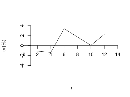
We verify that there is a “tendency” for the absolute value of the error to decrease as the sample size \(n\) increases. We made \(1,000\) repetitions of this procedure in a statistical analysis program and the graphical result is given by:
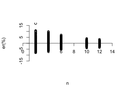
We observe that there is a tendency for the amplitudes of the relative errors to decrease with increasing sample size \(n\).
-
3.2.9 Considering each cell of the table presented as a position of an individual cage, as in the following scheme:
Weight of females 1 2 3 4 5 6 7 8 9 10 11 12 13 14 15 16 17 18 19 20 Thus, we have \(20\) individual cages and we perform a systematic sampling. We draw a position and, with jumps \(r\) \(\approx \) \(N / n\), we draw the sample of size \(n\). For example, for \(n=2\) we have \(r=20/2\) \(=\) \(10\). Thus, we draw an element among the first \(10\) and then jump \(r=10\) units to the next one.
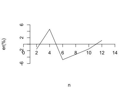
To obtain the relative errors for each sample size, we built the following table containing the samples drawn of each size systematically and the estimate of the mean. The relative error was estimated according to the procedure described in exercise 3.2.1. In the samples of size \(n=2\) the elements \(9\) and \(19\) were drawn. Note that \(r=10\) and the drawing among the first ten elements resulted in the value \(9\). For \(n=4\), the drawing was \(1\), \(6\), \(11\), \(16\). In this case \(r=5\) and the element drawn among the first \(5\) was \(1\), resulting in this sample. For \(n=6\) the drawing was \(3\), \(6\), \(9\), \(12\), \(15\), \(18\), with \(r=3\). For \(n=10\) the drawing was \(2\), \(4\), \(6\), \(8\), \(10\), \(12\), \(14\), \(16\), \(18\), \(20\), with \(r=2\). Finally, for \(n=12\) the drawing was \(1\), \(2\), \(3\), \(4\), \(5\), \(6\), \(7\), \(8\), \(9\), \(10\), \(11\), \(12\) with \(r=1\). It is important to emphasize that this method is not appropriate to be applied when \(n > N/2\), as in this last case of \(n=12\). The corresponding values, using the table above as a mask for the table with the original data and using the numbers drawn above, are presented in the following results table:
Size \((n)\) Sample
\(\bar {X}\) \(er\)% 2 17.44; 19.14
18.2900 \(-\)1.54% 4 18.77; 17.90; 21.71; 19.37
19.4375 4.63% 6 18.47; 17.90; 17.44; 17.37; 17.93; 16.99
17.6833 \(-\)4.81% 10 19.17; 18.40; 17.90; 19.38; 17.51; 17.37; 18.62; 19.37; 16.99; 18.30
18.3010 \(-\)1.49% 12 18.77; 19.17; 18.47; 18.40; 17.76; 17.90; 21.65; 19.38; 17.44; 17.51; 21.71; 17.37
18.7942 1.17% The corresponding graph is given by:
-
3.2.10 Uniform stratified sampling should be used when the population strata have approximately equal sizes, and proportional stratified sampling when these strata have very different sizes from each other. In proportional stratified sampling the sample stratum size is directly proportional to the population stratum size. Thus, the larger \(N_h\), the larger the sample size in that stratum \((n_h)\). Likewise, the expression used to size the sample stratum allows this analysis to be made. The corresponding expression is:
\(\seteqnumber{0}{3.}{0}\)\begin{align*} n_h=& \dfrac {N_h}{N} \times n. \end{align*}