Basic Statistics
8.2 Solutions
-
8.2.1 The mean, variance and standard deviation of this population are \(\mu \) \(=\) 2.3333, \(\sigma ^2\) \(=\) 1.5556 and \(\sigma \) \(=\) 1.2472. Let us first consider the samplings with replacement. For \(n=2\), we have
Samples \(\bar {X}\) \(S^2\) \(S\) 1, 1 1.0 0.0000 0.0000 1, 2 1.5 0.5000 0.7071 1, 4 2.5 4.5000 2.1213 2, 1 1.5 0.5000 0.7071 2, 2 2.0 0.0000 0.0000 2, 4 3.0 2.0000 1.4142 4, 1 2.5 4.5000 2.1213 4, 2 3.0 2.0000 1.4142 4, 4 4.0 0.0000 0.0000 Mean 2.3333 1.5556 0.9428 In this case, with \(n=2\) and sampling with replacement, we have that \(\sigma ^2_{\bar {X}}\) \(=\) 0.7778.
For \(n=3\), with replacement, we have:
Samples \(\bar {X}\) \(S^2\) \(S\) 1, 1, 1 1.0000 0.0000 0.0000 1, 1, 2 1.3333 0.3333 0.5774 1, 1, 4 2.0000 3.0000 1.7321 1, 2, 1 1.3333 0.3333 0.5774 1, 2, 2 1.6667 0.3333 0.5774 1, 2, 4 2.3333 2.3333 1.5275 1, 4, 1 2.0000 3.0000 1.7321 1, 4, 2 2.3333 2.3333 1.5275 1, 4, 4 3.0000 3.0000 1.7321 2, 1, 1 1.3333 0.3333 0.5774 2, 1, 2 1.6667 0.3333 0.5774 2, 1, 4 2.3333 2.3333 1.5275 2, 2, 1 1.6667 0.3333 0.5774 2, 2, 2 2.0000 0.0000 0.0000 2, 2, 4 2.6667 1.3333 1.1547 2, 4, 1 2.3333 2.3333 1.5275 2, 4, 2 2.6667 1.3333 1.1547 2, 4, 4 3.3333 1.3333 1.1547 4, 1, 1 2.0000 3.0000 1.7321 4, 1, 2 2.3333 2.3333 1.5275 4, 1, 4 3.0000 3.0000 1.7321 4, 2, 1 2.3333 2.3333 1.5275 4, 2, 2 2.6667 1.3333 1.1547 4, 2, 4 3.3333 1.3333 1.1547 4, 4, 1 3.0000 3.0000 1.7321 4, 4, 2 3.3333 1.3333 1.1547 4, 4, 4 4.0000 0.0000 0.0000 Mean 2.3333 1.5556 1.1093 In this case, with \(n=3\) and sampling with replacement, we have that \(\sigma ^2_{\bar {X}}\) \(=\) 0.5185161.
Let us now consider the samplings without replacement. For \(n=2\), we have
Samples \(\bar {X}\) \(S^2\) \(S\) 1, 2 1.5 0.5000 0.7071 1, 4 2.5 4.5000 2.1213 2, 4 3.0 2.0000 1.4142 Mean 2.3333 2.3333 1.4142 In this case, with \(n=2\) and sampling without replacement, we have that \(\sigma ^2_{\bar {X}}\) \(=\) 0.3889. For \(n=3\), it does not make sense in this case, since there is only one possible sample, \(\binom {N}{n}\) \(=\) \(\binom {3}{3}\) \(=\) \(1\).
-
a) The sampling distributions for \(\bar {X}\), \(S^2\) and \(S\) were presented above. For the case of \(\bar {X}\), the figures below refer to the cases with replacement of the distribution of \(\bar {X}\) for \(n=2\) and \(n=3\). We can observe that as \(n\) increases, the histogram resembles more the graph of a normal distribution. Of course, this is not very evident, since our example is only didactic so that we can carry out the sampling of all possible samples. In real populations, which are very large, and with sample sizes generally applied in practice, this manual process we did is impracticable and we use the theory to demonstrate it. The theorem behind this theory is the central limit theorem.
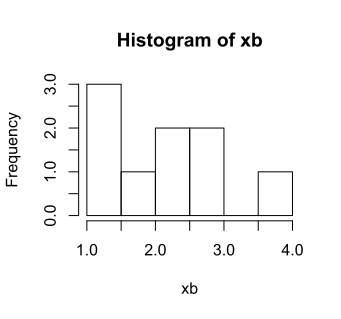
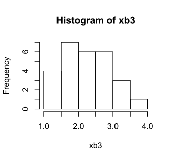
The mean at the end of each table is equivalent to the expectation of the corresponding estimator in each column. Thus, for \(n=2\), sampling with replacement, we have \(E(\bar {X})\) \(=\) 2.3333, \(E(S^2)\) \(=\) 1.5556 and \(E(S)\) \(=\) 0.9428. Still with sampling with replacement, for \(n=3\) we have: \(E(\bar {X})\) \(=\) 2.3333, \(E(S^2)\) \(=\) 1.5556 and \(E(S)\) \(=\) 1.1093. It is observed, by comparing the expectations with the respective parameters, that \(E(\bar {X})=\mu \) and \(E(S^2)=\sigma ^2\), but \(E(S)\ne \sigma \). The mean of the standard deviations in the respective sampling distributions mentioned are smaller than the value of the parameter \(\sigma \). The smaller the sample, the farther the expectation of the sample standard deviation was from the parametric value, in the sense of underestimating it. Thus, we conclude that \(\bar {X}\) and \(S^2\) are unbiased estimators of \(\mu \) and \(\sigma ^2\), respectively. On the other hand, the standard deviation is a biased estimator that underestimates the underlying parameter \(\sigma \).
In samples without replacement from finite populations, as in the case of the example for \(n=2\), we have that the only unbiased estimator is the sample mean \(\bar {X}\), since \(E(S^2)\ne \sigma ^2\) and \(E(S)\ne \sigma \). We know from the sampling distribution that when the sampling is without replacement from finite populations of size \(N\), then the observations are negatively correlated with each other; for this reason the sample variance \(S^2\) is a biased estimator of \(\sigma ^2\). We know that \(E(S^2)\) \(=\) \(N/(N-1)\sigma ^2\), which in this case is \(E(S^2)\) \(=\) \(3/2\times \) 1.5556 \(=\) 2.3333, which is exactly the result found in the example. The larger \(N\), the closer to \(1\) the multiplicative factor \(N/(N-1)\) becomes and, consequently, the smaller the bias.
-
b) The variances of the sample mean in each case are:
-
i) samples with replacement and \(n=2\): \(\sigma ^2_{\bar {X}}\) \(=\) 0.7778;
-
ii) samples with replacement and \(n=3\): \(\sigma ^2_{\bar {X}}\) \(=\) 0.5185;
-
iii) samples without replacement and \(n=2\): \(\sigma ^2_{\bar {X}}\) \(=\) 0.3889.
We know from the theory that the relations of the variance of \(\bar {X}\) in the sampling distribution with the population variance in the sampling distributions with and without replacement are
\(\seteqnumber{0}{8.}{0}\)\begin{align*} \sigma ^2_{\bar {X}} =& \dfrac {\sigma ^2}{n} &\textrm { and }&& \sigma ^2_{\bar {X}} =& \dfrac {\sigma ^2}{n}\dfrac {N-n}{N-1}, \end{align*} respectively. In samples with replacement its value for \(n=2\) is \(\sigma ^2_{\bar {X}}\) \(=\) 1.5556/2 \(=\) 0.7778 and for \(n=3\) it is \(\sigma ^2_{\bar {X}}\) \(=\) 0.5185, which are the values found directly in the sampling distribution. In the case of sampling without replacement, for \(n=2\), we have \(\sigma ^2_{\bar {X}}\) \(=\) 1.5556/2\(\times \) (3-2)/(3-1) \(=\) 0.3889, which was also the result obtained.
To answer the question of which sampling system leads to greater precision, we can consider the case of \(n=2\) and verify that the variance of the sample means is smaller in the sampling without replacement; therefore, this is the system with greater precision. Intuitively it is easy to see this, since when sampling with replacement we can draw the same population element more than once. Clearly, this repeated element or even all that are repeatedly drawn in the sample will not bring additional information that just one copy of them would not have added. In sampling without replacement, a drawn element cannot be drawn again and this does not happen. If, however, the population is very large relative to the sample size, the chance of repeating the draws in the samplings with replacement decreases with the increase of \(N\) relative to \(n\). Thus, the two systems (without and with replacement) become equivalent. This is clearly seen, since for fixed \(n\), \(\lim _{N\rightarrow \infty } (N-n)/(N-1)\) \(=\) \(1\), which makes the variances of the sample means of the two systems equal.
-
-
-
8.2.2 An interesting criterion to determine these estimators would be to minimize the sum of squares of these errors over all \(n\) pairs (\(x_i\), \(Y_i\)). This sum of squares is given by
\(\seteqnumber{0}{8.}{0}\)\begin{align*} \sum _{i=1}^{n}\epsilon _i^2 =& \sum _{i=1}^{n}\left (Y_i - \alpha - \beta x_i \right )^2. \end{align*} This method is called least squares and is easily obtained by differentiating this last expression with respect to the parameters \(\alpha \) and \(\beta \) and setting these derivatives equal to zero. Let us consider that we do not observe \(X\) yet, that is, instead of \(x_i\) we will use the random variable \(X_i\) from now on. We must minimize the sum of its squares \(\sum _{i=1}^{n}\epsilon _i^2\). Denoting this sum by \(Q\) we have
\(\seteqnumber{0}{8.}{0}\)\begin{align} \label {eb8:eq:143} Q=& \sum _{i=1}^{n}\epsilon _i^2 = \sum _{i=1}^{n} \left (Y_i-\alpha -\beta X_i\right )^2. \end{align}
Thus, the minimum can be obtained by calculus, differentiating \(Q\) with respect to the parameters \(\alpha \) and \(\beta \). The resulting functions are set equal to zero and solved for \(\alpha \) and \(\beta \), thus obtaining the least squares estimators. These derivatives are
\(\seteqnumber{0}{8.}{1}\)\begin{align*} \dfrac {\partial Q}{\partial \alpha } =& -2 \sum _{i=1}^{n} \left (Y_i-\alpha -\beta X_i\right )\\ \dfrac {\partial Q}{\partial \beta } =& -2 \sum _{i=1}^{n} \left (Y_i-\alpha -\beta X_i\right )X_i. \end{align*}
Setting these derivatives equal to zero and replacing \(\alpha \) and \(\beta \) by the respective estimators \(\hat {\alpha }\) and \(\hat {\beta }\), we have, after some simplifications, the so-called normal equations
\(\seteqnumber{0}{8.}{1}\)\begin{align} \label {eb14:eq:144} \left \{ \begin{array}{l} \displaystyle n\hat {\alpha } +\hat {\beta }\sum _{i=1}^{n} X_i = \displaystyle \sum _{i=1}^{n}Y_i \\ \\ \displaystyle \hat {\alpha } \sum _{i=1}^{n} X_i +\hat {\beta }\sum _{i=1}^{n} X_i^2 = \displaystyle \sum _{i=1}^{n}X_iY_i. \end {array} \right . \end{align}
Isolating \(\hat {\alpha }\) in the first expression of (8.2), we have
\(\seteqnumber{0}{8.}{2}\)\begin{align} \label {eb14:eq:145} \hat {\alpha } =& \dfrac {\displaystyle \sum _{i=1}^{n}Y_i}{n}- \hat {\beta }\dfrac {\displaystyle \sum _{i=1}^{n} X_i}{n} = \bar {Y}_.-\hat {\beta }\bar {X}_{.}. \end{align}
Substituting this result into the second expression of (8.2) and performing some simplification we obtain
\(\seteqnumber{0}{8.}{3}\)\begin{align*} \left [\sum _{i=1}^{n}X_i^2 - \dfrac {\displaystyle \left (\sum _{i=1}^{n} X_i \right )^2}{n}\right ] \hat {\beta }=& \sum _{i=1}^{n}X_iY_i - \dfrac {\displaystyle \sum _{i=1}^{n}X_i \sum _{i=1}^{n}Y_i}{n} \end{align*} which results in
\(\seteqnumber{0}{8.}{3}\)\begin{align} \label {eb14:eq:146} \hat {\beta }=& \dfrac {SPXY}{SQX}, \end{align} where \(SPXY\) represents the sum of products between \(X\) and \(Y\) and \(SQX\), the sum of squares of \(X\), given, respectively, by
\(\seteqnumber{0}{8.}{4}\)\begin{align} \label {eb14:eq:147} \left \{ \begin{array}{lc} SPXY= \displaystyle \sum _{i=1}^{n}X_iY_i - \dfrac {\displaystyle \sum _{i=1}^{n}X_i \sum _{i=1}^{n}Y_i}{n}, & \textrm { (a)} \\ SQX=\displaystyle \sum _{i=1}^{n}X_i^2 - \dfrac {\displaystyle \left (\sum _{i=1}^{n} X_i \right )^2}{n}, & \,\,\textrm { (b).} \end {array} \right . \end{align}
Thus, the function \(Q\) represents the sum of squares of errors. Therefore, assuming that the residual \(e_i\) is the predictor of the error \(\epsilon _i\), then the sum of its squares is called the residual sum of squares and is given by
\(\seteqnumber{0}{8.}{5}\)\begin{align*} \sum _{i=1}^{n} e_i^2 =& SQRes =\sum _{i=1}^{n} \left (Y_i-\hat {\alpha }-\hat {\beta }X_i\right )^2. \end{align*} This is the sum of squares of the residuals, where the residuals are the predictors of the random errors. The word predictor was used because the errors are random variables, not parameters. Thus, predictors are obtained, not estimators of random variables. For parameters, estimators are obtained. This sum of squares is associated with \(n-2\) degrees of freedom (two parameters). Therefore, the variance of the residuals, called the residual mean square, is given by
\(\seteqnumber{0}{8.}{5}\)\begin{align*} S^2 =& QMRes=\dfrac {1}{n-2}\sum _{i=1}^{n} e^2_i=\dfrac {SQRes}{n-2}. \end{align*}
The method-of-moments estimator of \(\sigma ^2\) is, therefore,
\(\seteqnumber{0}{8.}{5}\)\begin{align*} \hat {\sigma }^2 =& QMRes. \end{align*}
-
8.2.3 The sample mean and variance are given, respectively, by \(\bar {X}\) \(=\) 10.158 and \(S^2\) \(=\) 4.480996. According to normal theory, the sample mean when the variance is known, as is the case, has a normal distribution with mean \(\mu _{\bar {X}}\) \(=\) \(\mu \) and variance \(\sigma ^2_{\bar {X}}\) \(=\) \(\sigma ^2/n\). Using this result, we can obtain the confidence interval for \(\mu \) through the following expression:
\(\seteqnumber{0}{8.}{5}\)\begin{align*} CI_{1-\alpha }(\mu ):\, \bar {X} \pm Z_{\alpha /2}\frac {\sigma }{\sqrt {n}}, \end{align*} where \(Z_{\alpha /2}\) is the upper quantile \(100\alpha /2\%\) of the standard normal distribution. With \(\alpha =0.05\), we have that \(Z_{0.025}=\)1.96. Thus, with \(\bar {X}\) \(=\) 10.158, \(n=10\) and \(\sigma ^2=3\), we have
\(\seteqnumber{0}{8.}{5}\)\begin{align*} CI_{1-\alpha }(\mu ): & 10.158 \pm 1.96\times \frac {\sqrt {3}}{\sqrt {10}}\\ & 10.158 \pm 1.0735, \end{align*} which results in
\(\seteqnumber{0}{8.}{5}\)\begin{align*} CI_{1-\alpha }(\mu ): & [9.0844,\,\, 11.2315]. \end{align*}
Thus, we have a confidence of \(95\%\) that the true mean \(\mu \) of the population is a value in the interval between 9.0844 and 11.2315. We should be aware that a parameter is a constant and once the interval is realized, there was a hit (the interval covered the true value) or an error (the interval did not cover the true value). Therefore, the probability is \(0\) or \(1\). What we state is that we are \(95\%\) confident that we made the correct inference, that is, that \(\mu \) is a value among the possible candidates determined by the interval. Thus, \(95\%\) refers to a probability relative to our uncertainty in view of the phenomenon being under sampling and possessing randomness involved. In the estimation process when we repeat a large number of times, tending to infinity, on average \(100(1-\alpha )\%\) of our obtained intervals cover the true parameter under estimation, in this case, \(\mu \). Since we have only one of these results, we have a “confidence” of \(95\%\) that we are in one of these cases of hits.
-
8.2.4 The hypothesis of interest is given by:
\(\seteqnumber{0}{8.}{5}\)\begin{align*} H_0:\, \mu =& 10 &\textrm { vs }&& H_1:\, \mu \ne & 10. \end{align*}
The sample mean and variance are:
\(\seteqnumber{0}{8.}{5}\)\begin{align*} \bar {X}=& 10.158 &\textrm { and }&& S^2=& 4.480996. \end{align*}
The test statistic:
\(\seteqnumber{0}{8.}{5}\)\begin{align*} Z_c=& \dfrac {\bar {X}- \mu _0}{\dfrac {\sigma }{\sqrt {n}}}=\dfrac {10.158-10}{\sqrt {\dfrac {3}{10}}}=0.29. \end{align*}
The critical region (region of rejection of the null hypothesis), knowing that \(Z_{0.025}=\)1.96, is given by:
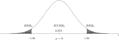
Since the value of \(Z_c\) belongs to the non-rejection region of the hypothesis, by the normal test, with \(95\%\) confidence, the null hypothesis should not be rejected, that is, we conclude that there is no reason to state that the population mean differs from \(10\).
Alternatively, we can use the confidence interval to perform the same hypothesis test. The general logic is to verify whether the hypothesized value belongs or not to the constructed confidence interval. If it is a value of the interval, as in the present case, the null hypothesis should not be rejected at the adopted confidence level. Otherwise, the null hypothesis is rejected.
In scientific practice we prefer to follow a simple strategy. We apply the test and verify whether there is statistical significance, that is, we verify whether the hypothesis should be rejected. If it is rejected, we obtain the confidence interval to estimate the effect size.