Basic Statistics
6.2 Solutions
-
6.2.1 The underlying distribution of the melting point \(X\) is the continuous uniform, with parameters \(\alpha =100\) and \(\beta =125\). For \(x\) \(\in \) \([100,\,125]\) the probability density and distribution functions are:
\(\seteqnumber{0}{6.}{0}\)\begin{align*} f(x;\alpha =100,\beta =125) =& \dfrac {1}{25} &\textrm { and }&&F(x;\alpha =100,\beta =125) =& \dfrac {x-100}{25}. \end{align*} Thus, the requested probabilities are:
-
a) \(P(108<X<122)=P(108<X<122)=F(122)-F(108)\) \(=\) \((122-100)/25-(108-100)/25\) \(=\) 0.88\(-\)0.32 \(=\) 0.56 \(=\) \(56\%\).
-
b) \(P(X>115)=1-F(115)=1-(115-100)/25=\)1\(-\)0.60=40%.
-
-
6.2.2 The distribution of the efficiency \(X\) underlying is the continuous uniform on \([0,\,100]\). The selling price is discretized into four real values \(P_1\), \(P_2\), \(P_3\), and \(P_4\), whose probabilities depend on the division into \(4\) classes of values of the underlying variable \(X\). The distribution function of \(X\) is \(F(x;0,100)=x/100\). Thus, the probability of \(X\) producing a value in the first class is: \(P(X<20)=F(20)=\)0.20. Likewise, for class \(2\), we have \(P(20\le X<50)\) \(=\) \(F(50)-F(20)\) \(=\) 0.50\(-\)0.20 \(=\) 0.30. For class \(3\), \(P(50\le X<80)\) \(=\) 0.30 and for class \(4\), \(P(X\ge 80)\) \(=\) \(1-F(80)\) \(=\) 0.20. These probabilities can be seen as the probabilities associated with each of the \(4\) prices and are denoted by \(P(P_i.)\). The expected value of the selling price \(P\) (average price) is
\(\seteqnumber{0}{6.}{0}\)\begin{align*} E(P) =& \sum _{i=1}^{4} P_i \times P(P_i)=0.2P_1+0.3P_2+0.3P_3+0.2P_4. \end{align*} Therefore, the answers to the questions asked are:
-
a) The average profit (L) per unit is, therefore,
\(\seteqnumber{0}{6.}{0}\)\begin{align*} L =& E(P) - C=0.2P_1+0.3P_2+0.3P_3+0.2P_4-C. \end{align*}
-
b) With \(C=10\) and \(P_1=0\) (discard), \(P_2=P_3/2=P_4/4\) we have the average price given by
\(\seteqnumber{0}{6.}{0}\)\begin{align*} E(P) =& 0.2P_1+0.3P_2+0.3P_3+0.2P_4=0.3P_2+0.3\times 2P_2+0.2\times 4P_2\\ =& 1.7P_2. \end{align*} The average profit per component is
\(\seteqnumber{0}{6.}{0}\)\begin{align*} L =& E(P) - C=1.7P_2-10. \end{align*} To answer the first question, we have that 1.7\(P_2-10=2\), which gives \(P_2=\)7.06 m.u. and, therefore, the prices \(P_3\) and \(P_4\) are \(P_3=\)14.12 m.u. and \(P_4=\)28.24 m.u., respectively.
To answer the second question we have that 1.7\(P_2-10>0\), which results in \(P_2=\)5.88 and, therefore, in \(P_3=\)11.76 and \(P_4=\)23.53 m.u. so as not to have losses.
-
-
6.2.3 The exponential model for the total daily rainfall in mm with parameter \(\lambda =\)0.0696:
-
a) The mean value is given by \(1/\lambda \), thus, \(\mu _X=\)1/0.0696 \(=\) 14.3678 mm. We could obtain this result by the general method, which, in fact, gave rise to this expression for the mean of the exponential. For this case, this process would be
\(\seteqnumber{0}{6.}{0}\)\begin{align*} E(X) =& \int _{0}^{\infty } x\times 0.0696e^{-0.0696x}dx=14.3678. \end{align*}
-
b) We will use the distribution function, which is \(F(X)\) \(=\) \(1-e^{-0.0696x}\), to compute the probabilities of this item and the following ones. Thus, \(P(X>25)\) \(=\) \(1-F(25)\) \(=\) \(1-(1-e^{-0.696\times 25})\) \(=\) 0.1755 \(=\) 17.55%.
-
c) \(P(X<5)\) \(=\) \(F(5)\) \(=\) \(1-e^{-0.696\times 5}\) \(=\) 0.2939 \(=\) 29.39%.
-
d) \(P(10< X< 18)=F(18)-F(10)=\)0.18\(-\)0.10=0.08=8%.
-
-
6.2.4 The mean (first moment) of the exponential is \(1/\lambda \). The estimator of the mean (of the first moment) is the sample mean \(\bar {X}\) in a sample of size \(n\). Thus, a method-of-moments estimator is given by
\(\seteqnumber{0}{6.}{0}\)\begin{align*} \bar {X} =& \dfrac {1}{\hat {\lambda }}\\ \hat {\lambda }=& \dfrac {1}{\bar {X}}. \end{align*} A second estimator can be obtained by equating the second moments centered on the mean (variance) of the population and of the sample. The variance of an exponential variable is \(1/\lambda ^2\). Thus, using the same reasoning we have that \(1/\hat {\lambda }^2=S^2\), which results in
\(\seteqnumber{0}{6.}{0}\)\begin{align*} \hat {\lambda } =& \dfrac {1}{\sqrt {S^2}}. \end{align*} Obviously, between the two estimators, there must be (and there is) one better than the other. Later, we will see some properties that allow us to choose between them by some optimality criterion.
-
6.2.5 Maximum likelihood estimator:
-
a) The likelihood function of the exponential distribution is
\(\seteqnumber{0}{6.}{0}\)\begin{align*} L(\lambda ;x_i)=& \prod _{i=1}^n f(x_i)\\ =&\prod _{i=1}^n \lambda e^{-\lambda x_i}\\ =& \lambda ^n e^{-\lambda \sum _{i=1}^n x_i}. \end{align*}
Taking the natural logarithm of \(L(\lambda ;x_i)\), we have
\(\seteqnumber{0}{6.}{0}\)\begin{align*} \ln L(\lambda ;x_i)=& n\ln (\lambda )-\lambda \sum _{i=1}^n x_i. \end{align*}
We differentiate \(\ln L(\lambda ;x_i)\) with respect to the parameter \(\lambda \), set it equal to zero, solve the resulting equation, and obtain the maximum likelihood estimate. Thus,
\(\seteqnumber{0}{6.}{0}\)\begin{align*} \dfrac {d \ln L(\lambda ;x_i)}{d \lambda }=& \dfrac {n}{\lambda } - \sum _{i=1}^n x_i, \end{align*} which, when set equal to zero, is
\(\seteqnumber{0}{6.}{0}\)\begin{align*} \dfrac {n}{\hat {\lambda }} - \sum _{i=1}^n x_i=&0\\ \dfrac {n}{\hat {\lambda }} =&\sum _{i=1}^n x_i\\ \hat {\lambda }=& \dfrac {n}{\displaystyle \sum _{i=1}^n x_i}= \dfrac {1}{\bar {x}}. \end{align*}
Thus, substituting the realizations of the random variables by the random variables themselves, we have that \(\hat {\lambda }\) \(=\) \(1/\bar {X}\) is the maximum likelihood estimator of the parameter \(\lambda \) of the exponential distribution.
-
b) We verify that the method-of-moments estimator (based on the first moment, the mean) and the maximum likelihood estimator of \(\lambda \) of the exponential are the same, that is, they are equal to the sample mean in a sample of size \(n\) from this distribution.
-
-
6.2.6 The probabilities of the standard normal can be obtained directly from the table or with some simple elementary operations of the values obtained directly from the table. In the figures that follow, the value of the desired probability will be hatched (black or black and gray) and the tabulated value in gray, when it is possible to do so. The normal table with \(P(0<Z<z|z)\) is presented below:
\(Z_t\) 0 1 2 3 4 5 6 7 8 9 0.0 0.0000 0.0040 0.0080 0.0120 0.0160 0.0199 0.0239 0.0279 0.0319 0.0359 0.1 0.0398 0.0438 0.0478 0.0517 0.0557 0.0596 0.0636 0.0675 0.0714 0.0753 0.2 0.0793 0.0832 0.0871 0.0910 0.0948 0.0987 0.1026 0.1064 0.1103 0.1141 0.3 0.1179 0.1217 0.1255 0.1293 0.1331 0.1368 0.1406 0.1443 0.1480 0.1517 0.4 0.1554 0.1591 0.1628 0.1664 0.1700 0.1736 0.1772 0.1808 0.1844 0.1879 0.5 0.1915 0.1950 0.1985 0.2019 0.2054 0.2088 0.2123 0.2157 0.2190 0.2224 0.6 0.2257 0.2291 0.2324 0.2357 0.2389 0.2422 0.2454 0.2486 0.2517 0.2549 0.7 0.2580 0.2611 0.2642 0.2673 0.2704 0.2734 0.2764 0.2794 0.2823 0.2852 0.8 0.2881 0.2910 0.2939 0.2967 0.2995 0.3023 0.3051 0.3078 0.3106 0.3133 0.9 0.3159 0.3186 0.3212 0.3238 0.3264 0.3289 0.3315 0.3340 0.3365 0.3389 1.0 0.3413 0.3438 0.3461 0.3485 0.3508 0.3531 0.3554 0.3577 0.3599 0.3621 1.1 0.3643 0.3665 0.3686 0.3708 0.3729 0.3749 0.3770 0.3790 0.3810 0.3830 1.2 0.3849 0.3869 0.3888 0.3907 0.3925 0.3944 0.3962 0.3980 0.3997 0.4015 1.3 0.4032 0.4049 0.4066 0.4082 0.4099 0.4115 0.4131 0.4147 0.4162 0.4177 1.4 0.4192 0.4207 0.4222 0.4236 0.4251 0.4265 0.4279 0.4292 0.4306 0.4319 1.5 0.4332 0.4345 0.4357 0.4370 0.4382 0.4394 0.4406 0.4418 0.4429 0.4441 1.6 0.4452 0.4463 0.4474 0.4484 0.4495 0.4505 0.4515 0.4525 0.4535 0.4545 1.7 0.4554 0.4564 0.4573 0.4582 0.4591 0.4599 0.4608 0.4616 0.4625 0.4633 1.8 0.4641 0.4649 0.4656 0.4664 0.4671 0.4678 0.4686 0.4693 0.4699 0.4706 1.9 0.4713 0.4719 0.4726 0.4732 0.4738 0.4744 0.4750 0.4756 0.4761 0.4767 2.0 0.4772 0.4778 0.4783 0.4788 0.4793 0.4798 0.4803 0.4808 0.4812 0.4817 2.1 0.4821 0.4826 0.4830 0.4834 0.4838 0.4842 0.4846 0.4850 0.4854 0.4857 2.2 0.4861 0.4864 0.4868 0.4871 0.4875 0.4878 0.4881 0.4884 0.4887 0.4890 2.3 0.4893 0.4896 0.4898 0.4901 0.4904 0.4906 0.4909 0.4911 0.4913 0.4916 2.4 0.4918 0.4920 0.4922 0.4925 0.4927 0.4929 0.4931 0.4932 0.4934 0.4936 2.5 0.4938 0.4940 0.4941 0.4943 0.4945 0.4946 0.4948 0.4949 0.4951 0.4952 2.6 0.4953 0.4955 0.4956 0.4957 0.4959 0.4960 0.4961 0.4962 0.4963 0.4964 2.7 0.4965 0.4966 0.4967 0.4968 0.4969 0.4970 0.4971 0.4972 0.4973 0.4974 2.8 0.4974 0.4975 0.4976 0.4977 0.4977 0.4978 0.4979 0.4979 0.4980 0.4981 2.9 0.4981 0.4982 0.4982 0.4983 0.4984 0.4984 0.4985 0.4985 0.4986 0.4986 3.0 0.4987 0.4987 0.4987 0.4988 0.4988 0.4989 0.4989 0.4989 0.4990 0.4990 3.1 0.4990 0.4991 0.4991 0.4991 0.4992 0.4992 0.4992 0.4992 0.4993 0.4993 3.2 0.4993 0.4993 0.4994 0.4994 0.4994 0.4994 0.4994 0.4995 0.4995 0.4995 3.3 0.4995 0.4995 0.4995 0.4996 0.4996 0.4996 0.4996 0.4996 0.4996 0.4997 3.4 0.4997 0.4997 0.4997 0.4997 0.4997 0.4997 0.4997 0.4997 0.4997 0.4998 3.5 0.4998 0.4998 0.4998 0.4998 0.4998 0.4998 0.4998 0.4998 0.4998 0.4998 3.6 0.4998 0.4998 0.4999 0.4999 0.4999 0.4999 0.4999 0.4999 0.4999 0.4999 3.7 0.4999 0.4999 0.4999 0.4999 0.4999 0.4999 0.4999 0.4999 0.4999 0.4999 3.8 0.4999 0.4999 0.4999 0.4999 0.4999 0.4999 0.4999 0.4999 0.4999 0.4999 3.9 0.5000 0.5000 0.5000 0.5000 0.5000 0.5000 0.5000 0.5000 0.5000 0.5000 -
a) The probability \(P(Z>\)1.50\()\) is illustrated in the figure below, in black. In gray is the area that the table provides:
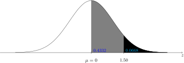
Thus, \(P(Z> \)1.50\()=\)0.5\(-P(0<Z< \)1.50\()=\)0.5\(-\)0.4332=0.0668=6.68%.
-
b) The probability \(P(Z>-\)1.50\()\) is illustrated in the figure below, in black and gray colors (all hatched area). In gray is the area that the table provides (by symmetry):
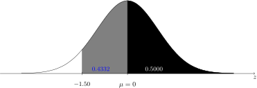
Thus, \(P(Z>-\)1.50\()=\)0.5+ P(\(-\)1.50
-
c) The probability \(P(-\)1.50
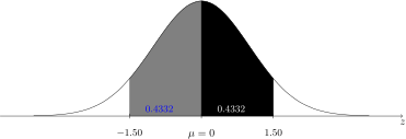
Thus, \(P(-\)1.50
-
d) The probability \(P(-\)1.96
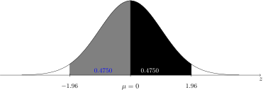
Thus, \(P(-\)1.96
-
e) The probability \(P(Z>0)\) is illustrated in the figure below, in black (obtained directly from the properties of the standard normal):
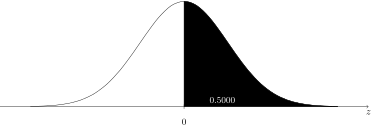
Thus, \(P(Z>0)=\)0.50=50%.
-
f) The probability \(P(\)1.30
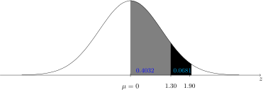
Thus, \(P(\)1.30
-
-
6.2.7 To solve this exercise we must always find the area between \(0\) and the quantile (value) \(z\), the value of interest to be determined, since the table we will consult (presented above) contains the probability of the following event: \(P(0<Z<z)\). Remember that inside the table are these areas (probabilities) under the curve and the value \(z\) of the random variable \(Z\) is in the first column of the table, with the second decimal place in the first row.
-
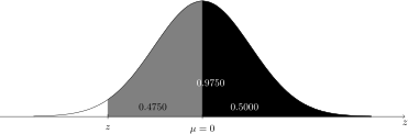
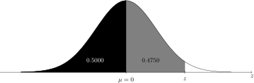
a) If \(P(Z>z)=\)0.9750, then \(P(z<Z<0)=\)0.9750\(-\)0.50=0.4750. Consulting the standard normal table, we locate the value 0.4750 inside it and verify that it corresponds to the value \(z=\)1.96. But since \(z<0\), then \(z=-\)1.96. See the illustrative figure. The hatched area, black and gray, corresponds to the value of the whole probability; the black area to \(P(Z>0)=\)0.50 and the gray area to the probability \(P(z<Z<0)=\)0.4750.
-
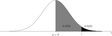
b) If \(P(Z>z)=\)0.0250, then \(P(0<Z<z)=\)0.50\(-\)0.0250=0.4750. Consulting the standard normal table, we locate the value 0.4750 inside it and verify that it corresponds to the value \(z=\)1.96. See the illustrative figure. The black area corresponds to the requested probability \(P(Z>z)=\)0.0250 and the gray area to the probability \(P(0<Z<z)=\)0.4750.
-
c) If \(P(Z<z)=\)0.9750, then \(P(0<Z<z)=\)0.9750\(-\)0.50=0.4750. Consulting the standard normal table, we locate the value 0.4750 inside it and verify that it corresponds to the value \(z=\)1.96. See the illustrative figure. The hatched area corresponds to the value of the whole probability; the black area to the probability \(P(Z<0)=\)0.50 and the gray area to \(P(0<Z<z)=\)0.4750.
-
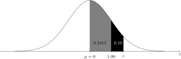
d) \(P(\)1.00\(<Z\le z)=\)0.10, then \(P(0<Z<1)+P(1<Z\le z)=\)0.3413\(+\)0.10=0.4413. Then, we can say that the area under the curve between \(0\) and \(z\) is equal to 0.4413. Thus, \(P(0<Z\le z)=\)0.4413. This probability value corresponds to the value \(z=\)1.57, without interpolation, that is, taking the closest value in the table. The gray colored area corresponds to the probability \(P(0<Z<1)=\)0.3413 and the entire hatched area (gray+black) to the probability \(P(0<Z\le z)=\)0.4413.
-
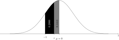
e) \(P(-1<Z< z)=\)0.20, then \(P(z<Z<0)=P(-1<Z<0)-\) 0.2000=0.3413\(-\)0.2000=0.1413. Then, we can say that the area under the curve between \(z\) and \(0\) is equal to 0.1413. This probability value corresponds to the value \(z=-\)0.36, without interpolation, that is, taking the closest value in the table. The black colored area corresponds to the probability \(P(-1<Z<z)=\)0.20 and the gray+black area to the probability \(P(-1<Z<0)=\)0.3413. The gray area corresponds to the probability \(P(z<Z<0)=\)0.1413. See the illustrative figure.
-
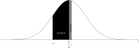
f) \(P(-1<Z< z)=\)0.40, then \(P(0<Z< z)=\)0.40\(-P(-1<Z<0)=\)0.40\(-\)0.3413=0.0587. Then, we can say that the area under the curve between \(z\) and \(0\) is equal to 0.0587. This probability value corresponds to the value \(z=\)0.15, without interpolation, that is, taking the closest value in the table. The black colored area corresponds to the probability \(P(-1<Z< 0)=\)0.3413 and the gray area to the probability \(P(0<Z<z)=\)0.0587. See the illustrative figure.
-
-
6.2.8 If the slaughter weight of the rabbits \(X \sim N(\mu =\)2.60, \(\sigma ^2=\)0.04\()\), then we can solve the questions presented as follows:
-
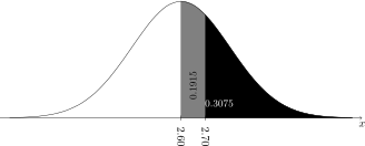
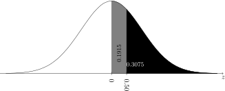
a) If \(P(X>\)2.70\()= P[Z>(\)2.70-2.60\()/0.20]=P(Z>\)0.50\()\) \(=\) 0.50\(-\)0.1915 \(=\) 30.75%. There is an equivalence between the areas under any normal curve and the areas under the standard normal curve, whose limits that delineate these regions are obtained by standardizing the limits of the original variable that limit the regions that determine the desired probabilities. In this example, the value of \(X\) of 2.70 that limits the region \(X>\)2.70 is equivalent in the standardized scale to the value of \(Z\) of 0.50. The general form for standardizing a value \(X_c\) of a variable \(X\) is given by
\(\seteqnumber{0}{6.}{0}\)\begin{align*} Z_c=& \dfrac {X_c-\mu }{\sigma }. \end{align*}
In the two graphs below we present the probability (area) under the normal \(N(\mu =\)2.60, \(\sigma ^2=\)0.04\()\) and the same probability in the standard normal \(N(\mu =0,\,\, \sigma ^2=1)\). The graph on the right is the standard normal, in which the value 0.50 represents the value 2.70 in the standardized scale. The black area represents the desired probability and the gray area the probability obtained from consulting the standard normal table (0.1915).
-
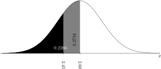
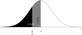
b) If \(P(X<\)2.45\()=P[Z<(\)2.45\(-\)2.60)/0.20\(]=P(Z<\)-0.75\()\) \(=\) 0.50\(-P(0<Z<\)0.75\()\) \(=\) 0.50\(-\)0.2734=22.66%.
In the two graphs below we present the probability (area) under the normal \(N(\mu =\)2.6; \(\sigma ^2=\)0.04\()\) and the same probability in the standard normal \(N(\mu =0;\,\, \sigma ^2=1)\). The graph on the right is the standard normal, in which the value \(-\)0.75 represents the value 2.45 in the standardized scale. The black area represents the desired probability and the gray area the probability obtained from consulting the standard normal table (0.2734).
-
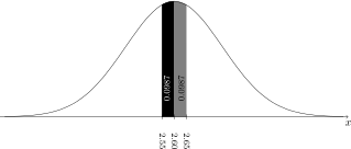
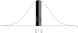
c) If P(2.55
In the two graphs below we present the probability (area) under the normal \(N(\mu =\)2.60, \(\sigma ^2=\)0.04\()\) and the same probability in the standard normal \(N(\mu =0,\,\, \sigma ^2=1)\). The second graph is the standard normal, in which the standardized values are \(-\)0.25 and 0.25 and represent the values 2.55 and 2.65 in the standardized scale.
-
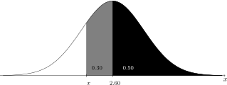
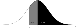
d) To obtain the weight \(x\) such that \(P(X>x)=\)0.80, we have that \(x<\)2.60 and that \(P(x<X<\)2.60\()=\)0.80\(-P(X>\)2.60\()\) \(=\) 0.3000. If \(z\) is the value corresponding to the standardized value of \(x\) in the standardized scale, that is, \(z=(x-\)2.60\()/\)0.20, we have that \(P(z<Z<0)=\)0.3000, for \(Z\sim N(0\), \(1)\). The graphs below illustrate these quantities in the original and standardized scales. The search in the table for the closest value to 0.30 (inside the table) results in \(-\)0.84 (by symmetry). Thus, the standardized value of \(x\) is \(z=-\)0.84. Using the destandardization formula we have
\(\seteqnumber{0}{6.}{0}\)\begin{align*} x =& \sigma z + \mu =-0.84\times 0.2+2.60=2.43, \end{align*} which is the desired value.
-
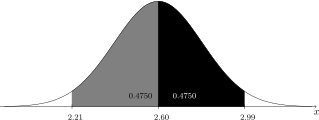
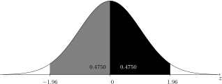
e) Obtain \(x\) such that \(P(\mu -x<X<\mu +x)=\)0.95. We have, considering that \(x>0\) and that \(\mu =\)2.60, that \(P(\)2.60\(<X<\)2.60\(+x)=\)0.95/2 \(=\) 0.4750. If \(z\) is the value corresponding to the standardized value of 2.60\(+x\) in the standardized scale, that is, \(z=(\)2.60\(+x-\)2.60\()/\)0.20 \(=\) \(5x\), we have that \(P(0<Z<z)=\)0.4750, for \(Z\sim N(0\), \(1)\). The graphs below illustrate these quantities in the original and standardized scales. The search in the table for the closest value to 0.4750 (inside the table) results in 1.96. Thus, the standardized value of \(\mu +x\) is \(z=\)1.96. Using the destandardization formula we have
\(\seteqnumber{0}{6.}{0}\)\begin{align*} \mu +x =& \sigma z + \mu =1.96\times 0.2+2.60=2.99. \end{align*} This implies that \(x\) \(=\) \(0.392\). Thus, the other value sought \(\mu -x\) is \(2.21\) kg. Therefore, the values sought are \(2.21\) and \(2.99\) kg.
-
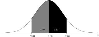
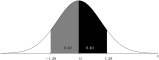
f) Similar to the previous case, we wish to obtain \(x\) such that \(P(\mu -x<X<\mu +x)=\)0.80. Assuming again that \(x>0\) and knowing that \(\mu =\)2.60, we have that \(P(\)2.60\(<X<\)2.60\(+x)=\)0.80/2 \(=\) 0.40. If \(z\) is the value corresponding to the standardized value of 2.60\(+x\) in the standardized scale, that is, \(z=(\)2.60\(+x-\)2.60\()/\)0.20 \(=\) \(5x\), we have that \(P(0<Z<z)=\)0.40, for \(Z\sim N(0\), \(1)\). The graphs below illustrate these quantities in the original and standardized scales. The search in the table for the closest value to 0.40 (inside the table) results in 1.96. Thus, the standardized value of \(\mu +x\) is \(z=\)1.28. Using the destandardization formula we have
\(\seteqnumber{0}{6.}{0}\)\begin{align*} \mu +x =& \sigma z + \mu =1.28\times 0.2+2.60=2.86. \end{align*} This implies that \(x\) \(=\) 0.256. Thus, the other value sought \(\mu -x\) is 2.34 kg. Therefore, the values sought are 2.34 and 2.86 kg.
-
g) Also for the rabbit case we have:
-
i) To find the weight limits of each class, let us consider, for illustration, the situation determined by the value \(x_1\) that delimits category \(E\) and that is the lower limit of category \(D\) (see figure below). In this case we will detail all the steps and make the corresponding graphs. For the remaining limits, we will not make all the corresponding graphs.
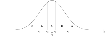
If \(P(X<x_1)=15\%\) and \(x_1\) can be standardized by
\(\seteqnumber{0}{6.}{0}\)\begin{align*} z_1=& \dfrac {x_1-\mu }{\sigma }=\dfrac {x_1-2.60}{0.20}. \end{align*}
Thus, \(P(X<x_1)=P(Z<z_1)=\)0.15; hence, \(P(z_1<Z<0)=\)0.5\(-\)0.15=0.35. If we consult the standard normal table, without interpolation, that is, looking for the value \(z_1\) whose area between \(z_1\) and \(0\) is approximately 0.35, we have \(z_1=-\)1.04 (check in the table). Thus, since \(z_1\) is the standardized value of \(x_1\), we can obtain \(x_1\) by substituting \(z_1=-\)1.04 into the previous standardization formula and solving for \(x_1\), as follows
\(\seteqnumber{0}{6.}{0}\)\begin{align*} -1.04=& \dfrac {x_1-2.60}{0.20} \textrm { hence,}\\ x_1=& 0.20\times (-1.04)+2.60=2.392 \textrm { kg}. \end{align*}
In the two graphs below we present the probability (area) under the normal \(N(\mu =\)2.60, \(\sigma ^2=\)0.04\()\) and the same probability in the standard normal \(N(\mu =0;\,\, \sigma ^2=1)\), corresponding to the event \(X<x_1\), for the values of \(x_1\) and \(z_1\), respectively. The second graph is the standard normal. Note that \(z_1\) is negative (\(-\)1.04).
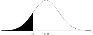
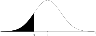
For the remaining values, which we will not illustrate with the corresponding graphs, we have:
If \(P(X<x_2)=15\%+20\%=35\%\), then \(x_2\) can be standardized by
\(\seteqnumber{0}{6.}{0}\)\begin{align*} z_2=& \dfrac {x_2-\mu }{\sigma }=\dfrac {x_2-2.60}{0.20}. \end{align*}
Thus, \(P(X<x_2)=P(Z<z_2)=\)0.35; hence, \(P(z_2<Z<0)=\)0.5\(-\)0.35=0.15. If we consult the standard normal table, without interpolation, that is, looking for the value \(z_2\) whose area between \(z_2\) and \(0\) is approximately 0.15, we have \(z_2=-\)0.39 (check in the table). Thus, since \(z_2\) is the standardized value of \(x_2\), we can obtain \(x_2\) by substituting \(z_2=-\)0.39 into the destandardization formula \(x_2=\sigma z_2+\mu \) as follows
\(\seteqnumber{0}{6.}{0}\)\begin{align*} x_2=& 0.20\times (-0.39)+2.60=2.552 \textrm { kg}. \end{align*}
For the limit \(x_3\), we have that \(P(X<x_3)=P(Z<z_3)=\)0.60; hence, \(P(0<Z<z_3)=\)0.65\(-\)0.5=0.10. If we consult the standard normal table, without interpolation, that is, looking for the value \(z_3\) whose area between \(0\) and \(z_3\) is approximately 0.10, we have \(z_3=\)0.25 (check in the table). Thus, since \(z_3\) is the standardized value of \(x_3\), we can obtain \(x_3\) by substituting \(z_3=\)0.25 into the destandardization formula \(x_3=\sigma z_3+\mu \) as follows
\(\seteqnumber{0}{6.}{0}\)\begin{align*} x_3=& 0.20\times 0.25+2.60=2.650 \textrm { kg}. \end{align*}
Finally, for the limit \(x_4\) we have that \(P(X<x_4)=P(Z<z_4)=\)0.90; hence, \(P(0<Z<z_4)=\)0.9\(-\)0.5=0.40. If we consult the standard normal table, without interpolation, that is, looking for the value \(z_4\) whose area between \(0\) and \(z_4\) is approximately 0.40, we have \(z_4=\)1.28 (check in the table). Thus, since \(z_4\) is the standardized value of \(x_4\), we can obtain \(x_4\) by substituting \(z_4=\)1.28 into the destandardization formula \(x_4=\sigma z_4+\mu \) as follows
\(\seteqnumber{0}{6.}{0}\)\begin{align*} x_4=& 0.20\times 1.28+2.60=2.856 \textrm { kg}. \end{align*}
Therefore, we should classify the rabbits into category \(E\) if their slaughter weight is less than 2.392 kg, into category \(D\) if their weight is between 2.392 kg and 2.552 kg, into category \(C\) if their weight is between 2.552 kg and 2.650 kg, into category \(B\) if their weight is between 2.650 kg and 2.856 kg, and into category \(A\) if their weight is greater than 2.856 kg.
-
ii) The average revenue is
\(\seteqnumber{0}{6.}{0}\)\begin{align*} \mu _R =& 2.1\times 0.15+ 3.0\times 0.20+5.0\times 0.25+5.2\times 0.30+2.5\times 0.10\\ =& 3.975. \end{align*} If the average cost is \(C=\)2.60, then the expected average profit is \(\mu _R-C\) \(=\) 1.375 m.u. per rabbit.
-
-
-
6.2.9 The variable \(Y\) referring to the number of seeds that germinate has a binomial distribution with probability of success \(p=\)0.70 and \(n=5\). Thus, \(Y\) \(\sim \) Binomial\((p=\)0.70, \(n=5)\). Hence, the desired solutions are presented in sequence.
-
a) If we use the binomial distribution the desired probability is:
\(\seteqnumber{0}{6.}{0}\)\begin{align*} P(Y\ge 4)=& P(X=4)+P(X=5)\\ =& \binom {5}{4}\left (0.70\right )^4\left (0.30\right )^{5-4}+ \binom {5}{5}\left (0.70\right )^5\left (0.30\right )^{5-5}\\ =& 0.2734375+0.21875\\ =& 0.6367187 \end{align*}
The probability that at least \(4\) of the \(5\) seeds germinate is 63.67187%.
-
b) Let us consider that \(X\) is the number of pots with at least \(4\) germinated seeds (minimum of \(4\) plants). An experiment with \(m\) pots to be sown with \(5\) seeds will be carried out if there are at least \(30\) pots with \(4\) plants (at least \(4\) germinated seeds). Thus, \(X\) \(\sim \) Binomial\((\theta =\)0.6367187, \(m)\), where \(\theta \) \(=\) \(P(Y\ge 4)\) \(=\) 0.6367187 is the probability of success, that is, that a pot chosen at random and that has been sown with at least \(5\) seeds has at least \(4\) germinated seeds, and \(m\) is the sample size, unknown in this case. The probability required for the experiment to be carried out is \(95\%\) and can be stated as follows:
\(\seteqnumber{0}{6.}{0}\)\begin{align*} P(X\ge 30) =& \sum _{t=30}^{m} \binom {m}{t} \theta ^t(1-\theta )^{m-t}=0.95. \end{align*}
We want to determine \(m\), the sample size, so that this condition is met. This sample size is the number of pots that must be sown with \(5\) seeds so that at the beginning of the experiment we have at least \(30\) of them with at least \(4\) plants. We can solve this by trial and error. For example, if we start with \(m=50\) and calculate the previous probability we will have 0.7560, which is less than \(95\%\). If we increase to \(m=58\), we will have \(P(X\ge 30)\) \(=\) 0.9773, which exceeds \(95\%\). Thus, we repeat this process for \(m=55\) and obtained \(P(X\ge 30)\) \(=\) 0.9375 and for \(m=56\) and obtained \(P(X\ge 30)\) \(=\) 0.9547. Thus, we conclude that \(m=56\) pots are necessary to guarantee with 95.47% the probability of the desired event.
For a solution of this type, an R program was made using the uniroot function and the exact relationship between the binomial and beta distribution functions. If \(I_z(\alpha ,\beta )\) is the beta distribution function evaluated at \(z\) with parameters \(\alpha >0\) and \(\beta >0\), this relationship is given by
\(\seteqnumber{0}{6.}{0}\)\begin{align*} P(X\le x|m,\theta ) =& I_{1-\theta }(m-x,x+1). \end{align*} The R program is:
theta <- 0.6367187
# Using the exact relationship between the
# binomial and beta distributions given by:
# 1-pbinom(29,m,theta) = 1-pbeta(1-theta,x-29,30)
fx <- function(x) 1-pbeta(1-theta,x-29,30) - 0.95
m <- uniroot(fx,c(30,400))$root # 30 to 400 is the root interval
m
The result for \(m\) in this case was 55.7. Since \(m\) is an integer value, \(55\) pots are insufficient to guarantee the probability and, therefore, the value that must be adopted is \(m=56\), as previously stated.
For the level of the book, we can use a second strategy to determine this value. Let us consider the normal approximation of the binomial. Since \(X\) is a binomial variable with parameters \(\theta =\)0.6367187 and \(m\) (unknown), then if \(W\) corresponds to the continuous version of the variable \(X\), \(W\) \(\dot {\sim }\) \(N(\mu =\)0.6367187\(m\), \(\sigma ^2=\)0.231308\(m)\), where \(\dot {\sim }\) means “is approximately distributed as”. Approximately we have the following probabilistic correspondences:
\(\seteqnumber{0}{6.}{0}\)\begin{align*} P(X\ge 30) \cong & P(W\ge 29.5)=0.95, \end{align*} where the value \(30\) was adjusted to 29.5 in the continuous (normal) scale for a better approximation (continuity correction).
Therefore, if we use the normal scale we have:
\(\seteqnumber{0}{6.}{0}\)\begin{align*} P(W\ge 29.5)=& P\left (Z\ge \dfrac {29.5-0.6367187m}{\sqrt {0.231308m}}\right )=0.95. \end{align*} Denoting \(z_1\) \(=\) (29.5\(-\)0.6367187\(m)/\sqrt {0.231308m}\), we have that \(z_1\) is a value of the standard normal distribution that has area above it under the curve of \(95\%\), which indicates that \(z_1<0\). The scheme below illustrates the value \(z_1\) in the standard normal.
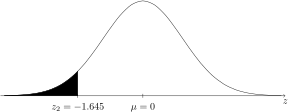
Therefore, \(z_1=-\)1.645 \(=\) (29.5\(-\)0.6367187\(m)/\sqrt {0.231308m}\), which must be solved for \(m\). Thus,
\(\seteqnumber{0}{6.}{0}\)\begin{align*} 29.5-0.6367187m =& -1.645\sqrt {0.231308m}. \end{align*}
Taking the squares of both sides, we have, after some simplifications
\(\seteqnumber{0}{6.}{0}\)\begin{align*} 870.25-37.5664m+0.4054107m^2 =& 0.6259252m\\ 0.4054107m^2-38.19233m+870.25=&0. \end{align*}
Solving the quadratic equation in \(m\) (number of pots), we have that
\(\seteqnumber{0}{6.}{0}\)\begin{align*} m =& \dfrac {38.19233\pm \sqrt {47.4193}}{\sqrt {0.8108214}} = \left \{\begin{array}{r} 38.61043 \\ 55.59609 \end {array} \right . \end{align*}
With \(m=\)38.61043, we have \(z_1=\)1.645, which corresponds to an area above of only \(5\%\). Now, if \(m=\)55.59609, the corresponding value of \(z_1\) is \(z_1=-\)1.645, providing both the sign and the probability correctly, that is, \(P(Z>-\)1.645)=0.95, as required. Hence, the only appropriate solution is 55.60. Since the final value of \(m\) is an integer value, the value \(55\) is insufficient and the final value must be \(m=56\), as obtained in the first method and as was already expected.
-
-
6.2.10 The probability of success is \(p=\)0.02 and the variable is a binomial, that is, \(X\) \(\sim \) binomial\((n=100\), \(p=\)0.02\()\), where \(X\) is the number of animals with swine fever in the random sample. This model is possible as long as we assume that the probability of success (event of interest) is not changed when sampling any animal and that the Bernoulli trials (samplings) are independent. The question then is to determine the probability of obtaining at least one diseased animal in the sample of size \(100\), that is, \(P(X\ge 1)\). Three different ways are proposed, one of which is an exact form that is the use of the binomial model. Below are the results obtained by the three requested ways.
-
a) Using the binomial model:
\(\seteqnumber{0}{6.}{0}\)\begin{align*} P(X\ge 1) =& 1-P(X=0)=1-\binom {100}{0}\times 0.02^0\times 0.98^100=1-0.1326196\\ =& 0.8673804. \end{align*} Thus, there is an 86.74% chance of sampling at least one animal with swine fever.
-
b) Using the binomial approximation we have that the parameter \(\lambda \) \(=\) \(np\) \(=\) \(100\times \) 0.02 \(=\) \(2\). Thus, the probability using the model \(P(X=x)\) \(\lambda ^xe^{-\lambda }/x!\) is:
\(\seteqnumber{0}{6.}{0}\)\begin{align*} P(X\ge 1) =& 1-P(X=0)=1-\dfrac {2^0e^{-2}}{0!}=1-0.1353353\\ =& 0.8646647. \end{align*} Thus, there is approximately an 86.47% chance of sampling at least one animal with swine fever.
-
c) Using the normal approximation, we have that \(\mu \) \(=\) \(np\) \(=\) \(2\) and \(\sigma ^2\) \(=\) \(np(1-p)\) \(=\) 1.96. Thus, using the continuity correction and denoting by \(Y\) the corresponding variable in the continuous (normal) scale, the probability is
\(\seteqnumber{0}{6.}{0}\)\begin{align*} P(X\ge 1) \approx & P(Y\ge 0.5)=P\left (Z\ge \dfrac {0.5-\mu }{\sigma }\right )=P\left (Z\ge \dfrac {0.5-2}{\sqrt {1.96}}\right )=P(Z\ge -1.07)\\ \approx & P( -1.07\le Z<0)+0.50=0.3577+0.50\\ \approx & 0.8577. \end{align*} Thus, there is approximately an 85.77% chance of sampling at least one animal with swine fever.
-
d) To compare the three values, we should consider that the binomial value is the exact value and, therefore, of reference. Thus, for the Poisson case, the absolute error was 0.0027157 downward (Poisson underestimated the true value) and the absolute relative error was 0.31%. For the normal, these values were 0.0096804 and 1.12%. Thus, the largest errors, in absolute or relative values, were with the normal. The normal approximation of the binomial is expected to be adequate when \(np>5\), which did not occur in this example, although the value found was not significantly far from the real value. When \(n\ge 100\) and \(p\le \)0.10, the Poisson distribution of the binomial is considered adequate (Leemis & Trivedi 1996), which occurred here, justifying the better estimates of the exact probability obtained in relation to the normal approximation of the binomial.
-