Basic Statistics
7.2 Solutions
-
7.2.1 According to the table provided and the probabilistic statements we have the following answers to the proposed exercises, considering the Student’s \(t\) distribution.
-
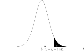
a) \(P(t>t_c)=\)0.05 with \(\nu =10\), so by consulting the miniature table of the Student’s \(t\) distribution we obtained \(t_c=\)1.812. See the scheme below, considering that \(\alpha =\)0.05 and \(1-\alpha =\)0.95. For this consultation we must find the \(\nu =10\) degrees of freedom in the first column and the value of the area to the right of the quantile (upper quantile) equal to \(\alpha =\)0.05 in the first row. At the intersection of the row and column corresponding to the mentioned values we find the value of \(t_c\), which is in this case 1.812.
-
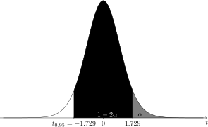
b) \(t_{0.95}\) with \(\nu =20-1\) is the same as \(P(t>t_{0.95})=\)0.95. Since we do not have the value 0.95 in the first row of the table, but we know that the Student’s \(t\) distribution is symmetric, we have that \(T_{0.95}=-t_{0.05}\). Thus, consulting the miniature table of the Student’s \(t\) distribution we obtained \(t_{0.05}=\)1.729. See the scheme below, considering that \(\alpha =\)0.05 and \(1-\alpha =\)0.95. For this consultation we must find the \(\nu =19\) degrees of freedom in the first column and the value of the area to the right of the quantile (upper quantile) equal to \(\alpha =\)0.05 in the first row. At the intersection of the row and column corresponding to the mentioned values we find the value \(t_{0.05}=\)1.729. Therefore, the answer to the case is \(t_{0.95}=-\)1.729.
In the figure, the black area has an area of \(1-2\alpha \) \(=\) 0.90 and the sum of the black and gray areas is 0.95 (index of the quantile \(t_{0.95}\)). The gray area is equivalent to 0.05. For this reason (symmetry), the \(t\) tables only have values less than 0.50 for their probabilities to the right of the upper quantile. For values of \(\alpha \) greater than 0.50 we use the property:
\(\seteqnumber{0}{7.}{0}\)\begin{align*} t_{\gamma ;\nu } =& -t_{1-\gamma ;\nu }, \end{align*} for 0.5\(<\gamma <\)1 and, thus, we can consult the table of upper quantiles of the Student’s \(t\) in the tables of the Books.
-
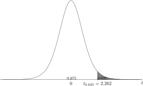
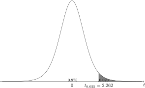
c) \(t_{0.025}\) with \(\nu =10-1=9\) degrees of freedom. If we consult the miniature table of the Student’s \(t\) distribution we have \(t_{0.025}=\)2.262. See the scheme below.
-
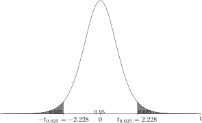
d) To determine \(t_{\alpha /2}\) given that \(P(-t_{\alpha /2} < t < t_{\alpha /2})=\)0.95, we have that \(\alpha =\)0.05 and \(\alpha /2=\)0.025. Consulting the table with \(\nu =10\) degrees of freedom we observe \(t_{0.025;\nu =10}=\)2.228. See illustrative scheme below.
-
e) We can write the expression \(\int _{t_c}^\infty f(t)dt=\)0.025 as \(P(t>t_c)=\)0.025, so \(t_c=t_{0.025;\nu =9}\). Thus, if we consult the miniature table of the Student’s \(t\) distribution we have \(t_c=\)2.262. See the scheme below and notice in a general way the different forms (notations) we have to obtain upper quantiles of the Student’s \(t\) distribution.
-
-
7.2.2 According to the table provided and the probabilistic statements we have the following answers to the proposed exercises, considering the chi-square distribution.
-
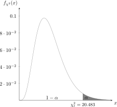
a) \(\chi ^2_{0.025;\nu =10}=\)20.483, according to the consultation we made in the miniature table of the chi-square distribution presented. We must use the probability 0.025 (column of the table) and the row corresponding to the degrees of freedom \(\nu =10\). See the figure below, where \(\chi ^2_t\) is the tabulated upper quantile of the chi-square distribution (tabulated chi-square).
-
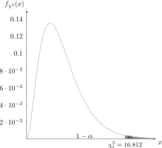
b) \(\chi ^2_{0.01;\nu =6}=\)16.812, according to the consultation we made in the miniature table of the chi-square distribution presented. We must use the probability 0.01 (column of the table) and the row corresponding to the degrees of freedom \(\nu =6\). See the figure below.
-
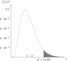
c) \(\chi ^2_{0.05;\nu =10}=\)18.307, according to the consultation we made in the miniature table of the chi-square distribution presented. We must use the probability 0.05 (column of the table) and the row corresponding to the degrees of freedom \(\nu =10\). See the figure below.
-
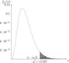
d) \(\chi ^2_{\alpha /2;\nu =8}=\chi ^2_{0.05;\nu =8}=\)15.507, since if \(P(\chi ^2\le \chi _{\alpha /2}^2)=\)0.95, it means that \(P(\chi ^2>\chi ^2_{\alpha /2})=\)0.05, being \(\alpha =\)0.10.
-
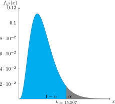
e) This case presents only a change of notation. We have that the announced definite integral determines an area under the curve (chi-square distribution with \(\nu =8\) degrees of freedom) between \(0\) and the value of \(k\) equal to 0.95. The area under the curve delimited by \(k\) and \(\infty \) represents \(5\%\). Therefore, \(k=\chi ^2_{0.05;\nu =8}=\)15.507. See illustrative scheme, with gray area for \(P(\chi ^2_{\nu =8}> k)=\)0.05 and cyan for \(P(\chi ^2_{\nu =8}\le k)=\)0.95.
-
-
7.2.3 According to the table provided and the probabilistic statements we have the following answers to the proposed exercises, considering the Snedecor’s \(F\) distribution.
-
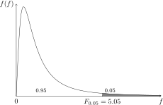
a) \(F_{0.05;\nu _1=5;\nu _2=5}=\)5.05, value resulting from consulting the miniature table of the \(F\) distribution. See illustrative figure below.
-
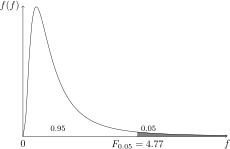
b) \(F_{0.05;\nu _1=9;\nu _2=5}=\)4.77, value resulting from consulting the miniature table of the \(F\) distribution. See illustrative figure below.
-
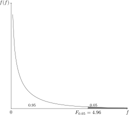
c) \(F_{0.05;\nu _1=1;\nu _2=10}=\)4.96, value resulting from consulting the miniature table of the \(F\) distribution. If we consult the Student’s \(t\) table we will see that \(t_{0.025;\nu =10}=\)2.228. If we take the square of the \(t\) quantile, we have 2.228\(^2\) \(=\) 4.963, which is equal to the tabulated value of \(F\). Thus, this relation is always valid, and can be stated in a general way by
\[F_{\alpha ;\nu _1=1,\nu _2}=t^2_{\alpha /2;\nu =\nu _2}.\]
Note that the probability above the quantile in the \(t\) is half \((\alpha /2)\) of that presented in the \(F\) distribution \((\alpha )\); the degrees of freedom \(\nu _1\) are always equal to \(1\); and the degrees of freedom of the \(t\), \(\nu \), is equal to \(\nu _2\) of the \(F\).
-
-
7.2.4 The variable \(X\) \(\sim \) exponential\((\lambda =1/120)\) refers to the lifetime of mango trees (plants). The mean and variance of the exponential are \(\mu =1/\lambda =120\) and \(\sigma ^2\) \(=\) \(1/\lambda ^2\) \(=\) \(120^2\), respectively. The mean of a sample of size \(n\), by the central limit theorem, has approximately a normal distribution, that is, \(\bar {X}\) \(\sim \) \(N(\mu \), \(\sigma ^2/n)\), which in this case results in \(\bar {X}\) \(\sim \) \(N(120\), \(144)\), for \(n\) \(=\) \(100\).
-
a) Determine \(P(\bar {X}>250)\):
\(\seteqnumber{0}{7.}{0}\)\begin{align*} P(\bar {X}>250) =& P\left (Z>\dfrac {250-120}{\sqrt {144}}\right )\\ =& P(Z>10.83)\\ =& 0. \end{align*}
-
b) Determine \(P(\bar {X}<60)\):
\(\seteqnumber{0}{7.}{0}\)\begin{align*} P(\bar {X}<60) =& P\left (Z<\dfrac {60-120}{\sqrt {144}}\right )\\ =& P(Z<-5)\\ =& 2.87\times 10^{-7}. \end{align*}
-
c) Determine \(P(100<\bar {X}<140)\):
\(\seteqnumber{0}{7.}{0}\)\begin{align*} P(100<\bar {X}<140) =& P\left (\dfrac {100-120}{\sqrt {144}}< Z< \dfrac {140-120}{\sqrt {144}}\right )\\ =& P(-1.67<Z<1.67)\\ =& 0.9044. \end{align*}
As can be seen, even using an approximation for the calculation, the probability of finding a sample presenting a sample mean very far from the mean value \(120\) is practically null. On the other hand, the vast majority, 90.44%, of the means in samples of size \(100\) lies between \(100\) and \(120\) years.
-
-
7.2.5 In the case of the exponential, we know that \(\bar {X}\) \(\sim \) gamma\((r=n\), \(n\lambda )\) in a random sample of size \(n\) from an exponential with parameter \(\lambda \), which for the exercise in question results in \(\bar {X}\) \(\sim \) gamma\((r=100\), \(5/6)\).
-
a) Determine \(P(\bar {X}>250)\):
\(\seteqnumber{0}{7.}{0}\)\begin{align*} P(\bar {X}>250) =& 1-P(\bar {X}\le 250)\\ =& 1 - \int _0^{250}\dfrac {5/6}{\Gamma (100)}(5/6\times u)^{100-1}e^{-5/6\times u} du\\ =& 1-1=0, \end{align*} using the command pgamma(250,shape=100,rate=5/6) of R to obtain the value of the gamma distribution function evaluated at \(250\).
Since both the exact value and the approximate value were equal to zero, within the limited precision of computer calculations, no errors were committed.
-
b) Determine \(P(\bar {X}<60)\):
\(\seteqnumber{0}{7.}{0}\)\begin{align*} P(\bar {X}<60) =& P(\bar {X}\le 60)\\ =& \int _0^{60}\dfrac {5/6}{\Gamma (100)}(5/6\times u)^{100-1}e^{-5/6\times u} du\\ =& 3.2\times 10^{-7}, \end{align*} with the help of R, command pgamma(60,shape=100,rate=5/6). The approximate value was 2.87\(\times 10^{-7}\) and the exact 3.2\(\times 10^{-7}\), so the absolute error was 3.3\(\times 10^{-8}\) in the sense of underestimating the exact value. The absolute relative error was 10.31%.
-
c) Determine \(P(100<\bar {X}<140)\):
\(\seteqnumber{0}{7.}{0}\)\begin{align*} P(100<\bar {X}<140) =& P(\bar {X}\le 140)-P(\bar {X}\le 100)\\ =& \int _0^{140}\dfrac {5/6}{\Gamma (100)}(5/6\times u)^{100-1}e^{-5/6\times u} du - \\ & - \int _0^{100}\dfrac {5/6}{\Gamma (100)}(5/6\times u)^{100-1}e^{-5/6\times u} du\\ =& 0.94685-0.0413149\\ =& 0.905535, \end{align*} using pgamma(140,shape=100,rate=5/6) - pgamma(100,shape=100,rate=5/6) of the program R. The absolute error was \(|\)0.9044\(-\)0.905535\(|\) \(=\) 0.001135 and the absolute relative percentage error 0.12534%, which can be considered quite small.
-
-
7.2.6 If \(X\) \(\sim \) binomial\((n\), \(p)\), then \(\hat {p}\) \(\dot {\sim }\) \(N(p\), \(p(1-p)/n)\), which in this case results in \(\hat {p}\) \(\dot {\sim }\) \(N(\)0.20, 0.0016\()\). Note that the random variable \(\hat {p}\) is a mean of Bernoulli variables, which are binary \((0\) or \(1)\), so the variable \(X\) \(=\) \(n\hat {p}\) (total of infested plants) can be approximated by a normal distribution. If in the continuous scale \(X\) is represented by \(Y\) \(=\) \(n\hat {p}\), then \(Y\) \(\dot {\sim }\) \(N(np\), \(np(1-p))\), using properties of the mean and variance when a random variable is multiplied by a constant, in this case \(n\). Therefore, \(Y\) \(\dot {\sim }\) \(N(20\), \(16)\). We will use, in all cases below, the continuity correction.
-
a) The probability of having infested plants between \(10\) and \(30\), excluding these two limits, is given approximately by
\(\seteqnumber{0}{7.}{0}\)\begin{align*} P(10<X<30)\approx & P(10.5<Y<29.5)=P\left (\dfrac {10.5-20}{4}<Z< \dfrac {29.5-20}{4} \right )\\ \approx & P(-2.38<Z<2.38)=0.9913-0.00866\\ \approx & 0.9827. \end{align*}
-
b) The probability that the number of infested plants is greater than \(40\) is:
\(\seteqnumber{0}{7.}{0}\)\begin{align*} P(X>40)\approx & P(Y>40.5)=P\left (Z>\dfrac {40.5-20}{4} \right )\\ \approx & P(Z>5.13)\\ \approx & 1.49\times 10^{-7}. \end{align*}
-
-
7.2.7 The random variable \(X\) \(\sim \) binomial\((n\), \(p)\), in this case, \(X\) \(\sim \) binomial\((100\), 0.20\()\). Using the exact binomial distribution we have:
-
a) The probability of having infested plants between \(10\) and \(30\), excluding these two limits, is given approximately by
\(\seteqnumber{0}{7.}{0}\)\begin{align*} P(10<X<30)=& P(X=11)+\cdots +P(X=29)\\ =& \binom {100}{11}\times 0.2^{11}\times 0.8^{99}+\cdots +\binom {100}{29}\times 0.2^{29}\times 0.8^{71}\\ =& 0.006878495+\cdots +0.008771228\\ =& 0.9830546. \end{align*} Since the approximate value was 0.9827, the absolute error is 0.0003546 and the absolute relative percentage error is 0.03607%.
-
b) The probability that the number of infested plants is greater than \(40\) is:
\(\seteqnumber{0}{7.}{0}\)\begin{align*} P(X>40) =&P(X=41)+\cdots +P(X=100)\\ =& 8.47\times 10^{-7}+\cdots +1.27\times 10^{-7}\\ =& 1.29\times 10^{-6} \end{align*} Since the approximate value was 1.49\(\times 10^{-7}\), the absolute error is 1.14\(\times 10^{-6}\) and the absolute relative percentage error is 88.45%. Although the relative error was very high, in absolute terms it is very small. Relative errors tend to be very high the smaller the exact reference value is, in general, since small errors on an absolute scale can represent a large portion of the true value, which is also very small (close to zero).
-
-
7.2.8 If the upper quantiles \(\chi ^2_{1-\alpha /2;\nu }\) and \(\chi ^2_{\alpha /2;\nu }\) of the chi-square distribution with \(\nu =n-1\) degrees of freedom and the probabilistic statement are considered
\(\seteqnumber{0}{7.}{0}\)\begin{align*} P\left (\chi ^2_{1-\alpha /2;\nu } \le \dfrac {\nu S^2}{\sigma ^2} \le \chi ^2_{\alpha /2;\nu }\right )=& 1-\alpha \\ P\left (\dfrac {\chi ^2_{1-\alpha /2;\nu }}{\nu S^2}\le \dfrac {1}{\sigma ^2} \le \dfrac {\chi ^2_{\alpha /2;\nu }}{\nu S^2}\right )=& 1-\alpha \\ P\left (\dfrac {\nu S^2}{\chi ^2_{1-\alpha /2;\nu }}\ge \sigma ^2 \ge \dfrac {\nu S^2}{\chi ^2_{\alpha /2;\nu }}\right )=& 1-\alpha \end{align*} one obtains
\(\seteqnumber{0}{7.}{0}\)\begin{align*} P\left (\dfrac {(n-1)S^2}{\chi ^2_{\alpha /2;\nu }}\le \sigma ^2 \le \dfrac {(n-1) S^2}{\chi ^2_{1-\alpha /2;\nu }}\right )=& 1-\alpha . \end{align*}
-
a) The previous probabilistic statement enables the construction of the \(1-\alpha \) confidence interval for the parameter \(\sigma ^2\). The resulting interval is
\(\seteqnumber{0}{7.}{0}\)\begin{align*} IC_{1-\alpha }\left (\sigma ^2\right ):\,\,\left [\dfrac {(n-1)S^2}{\chi ^2_{\alpha /2;\nu }}, \,\, \dfrac {(n-1) S^2}{\chi ^2_{1-\alpha /2;\nu }}\right ]. \end{align*}
-
b) Obtain limits in practice to estimate the parameter \(\sigma ^2\) and determine the precision of the estimation process. The logic is that if we repeat infinitely many times the sampling of size \(n\) from a normal population and construct this confidence interval, on average \(100(1-\alpha )\%\) of them will contain (cover) the true value \(\sigma ^2\) of the population variance. In many applications of genetics, both in animal and plant breeding and in quality control applications, among many other cases, this parameter is of fundamental importance.
-
-
7.2.9 Developing the expression presented, we have:
\(\seteqnumber{0}{7.}{0}\)\begin{align*} P\left (-t_{\alpha /2}\le \dfrac {\bar {X}-\mu }{\dfrac {S}{\sqrt {n}}}\le t_{\alpha /2}\right )=& 1-\alpha \\ P\left (-t_{\alpha /2}\dfrac {S}{\sqrt {n}}\le \bar {X}-\mu \le t_{\alpha /2}\dfrac {S}{\sqrt {n}}\right )= 1-\alpha & \\ P\left (-\bar {X}-t_{\alpha /2}\dfrac {S}{\sqrt {n}}\le -\mu \le -\bar {X}+ t_{\alpha /2}\dfrac {S}{\sqrt {n}}\right )=&1-\alpha \\ P\left (\bar {X}+t_{\alpha /2}\dfrac {S}{\sqrt {n}}\ge \mu \ge \bar {X}-t_{\alpha /2}\dfrac {S}{\sqrt {n}}\right )=&1-\alpha \\ P\left (\bar {X}-t_{\alpha /2}\dfrac {S}{\sqrt {n}}\le \mu \le \bar {X}+ t_{\alpha /2}\dfrac {S}{\sqrt {n}}\right )=& 1-\alpha . \end{align*}
-
a) The previous probabilistic statement enables the construction of the \(1-\alpha \) confidence interval for the parameter \(\mu \). The resulting interval is
\(\seteqnumber{0}{7.}{0}\)\begin{align*} IC_{1-\alpha }(\mu ):& \bar {X} \pm t_{\alpha /2;\nu } \dfrac {S}{\sqrt {n}}. \end{align*}
-
b) Obtain confidence intervals for the mean \(\mu \) of a normal population, which can be applied in routine work situations, such as in a sampling to determine what the production per ha of a eucalyptus plantation will be, as well as in scientific areas.
-
-
7.2.10 Let us consider \(X\) \(\sim \) \(N(\mu =\)9.5, \(\sigma ^2=9)\), then we can determine the distribution of \(\bar {X}\), \(\min (X_i's)\) and \(\max (X_i)\) in a sample of size \(n=20\).
-
a) In the case of \(\bar {X}\), we have that \(\bar {X}\) \(\sim \) \(N(\mu _{\bar {X}}=\)9.5 and \(\sigma ^2_{\bar {X}}=9/20)\). Therefore,
\(\seteqnumber{0}{7.}{0}\)\begin{align*} P(\bar {X} < 8) =& P\left (Z<\dfrac {8-9.5}{\frac {3}{\sqrt {20}}} \right )=P(Z<-2.24)\\ =& 0.0125=1.25\%. \end{align*}
-
b) If \(X_{(1)}\) \(=\) \(\min (X_i,i=1,\cdots ,n)\), we have that the distribution function, since the \(X_i\)’s are independent and identically distributed normal, is given by
\(\seteqnumber{0}{7.}{0}\)\begin{align*} F_{X_{(1)}}(x) =& P(X_{(1)}\le x)=1-\left [1-F_X(x)\right ]^{20}, \end{align*} where \(F_X(x)\) is the distribution function of a random variable \(X\) \(\sim \) \(N(\mu =\)9.5, \(\sigma ^2=9)\). We wish to obtain \(F_{X_{(1)}}(8)\). Thus,
\(\seteqnumber{0}{7.}{0}\)\begin{align*} F_{X_{(1)}}(8) =& P(X_{(1)}\le 8)=1-\left [1-P(X\le 8)\right ]^{20}\\ =& 1-\left [1-P\left (Z<\dfrac {8-9.5}{3}\right )\right ]^{20}\\ =& 1-\left [1-P\left (Z<-0.50\right )\right ]^{20}=1- \left (1-0.3085375\right )^{20}\\ =& 0.9993757. \end{align*} Thus, 99.94% of the normal samples of this population present a minimum value less than \(8\). We made an R program to show how this happens. In this program we performed \(1000000\) simulations and the estimate we obtained was 0.999409 (it will vary if you repeat this process, since it is a random process). See the program below:
mu <- 9.5
sig <- 3
x1 <- 11
#probabilidade exata mínimo
1 - (1 - pnorm(x1, mu, sig))^20
#probabilidade exata máximo
(pnorm(x1, mu, sig))^20
N <- 1000000
n <- 20
X <- matrix(c(rnorm(N * n, mu, sig)), N, n)
#estimativa da probabilidade
#exata do mínimo por simulação
x <- apply(X, 1, min)
length(x[x < x1]) / N
#estimativa da probabilidade
#exata do máximo por simulação
y <- apply(X, 1, max)
length(y[y < x1]) / N
-
c) If \(X_{(n)}\) \(=\) \(\max (X_i,i=1,\cdots ,n)\), we have that the distribution function, since the \(X_i\)’s are independent and identically distributed normal, is given by
\(\seteqnumber{0}{7.}{0}\)\begin{align*} F_{X_{(n)}}(x) =& P(X_{(n)}\le x)=\left [F_X(x)\right ]^{20}, \end{align*} where \(F_X(x)\) is the distribution function of a random variable \(X\) \(\sim \) \(N(\mu =\)9.5, \(\sigma ^2=9)\). We wish to obtain \(F_{X_{(n)}}(11)\). Thus,
\(\seteqnumber{0}{7.}{0}\)\begin{align*} F_{X_{(n)}}(11) =& P(X_{(n)}\le 11)=\left [P(X\le 11)\right ]^{20}\\ =& \left [P\left (Z<\dfrac {11-9.5}{3}\right )\right ]^{20}\\ =& \left [P\left (Z\le 0.50\right )\right ]^{20}= \left (0.6914625\right )^{20}\\ =& 0.0006242696. \end{align*} Thus, 0.062% of the normal samples of this population present a maximum value less than \(11\). In the simulation, whose previous program included the maximum case, it is 0.0606%, which is a reasonable estimate of the value found. Thus, there is a high probability that the samples of this normal population present maximums greater than \(11\), which is the complement to \(1\) of the value presented.
-