Basic Statistics
4.2 Solutions
-
4.2.1 Probability is an essential part of statistics for those who want to develop new methods of estimation and hypothesis testing. The foundation of any statistical method can only be achieved with the proper understanding of its theory, which is contained in the foundation of probabilistic theory. Thus, the adequate training of a statistician can only be achieved after learning and understanding the theories of this area. For those who intend only to make use of statistics, the concepts of probability are fundamental so that one can understand and apply methods of statistical inference.
-
4.2.2 The dendrogram (tree diagram) to help construct the sample space is:
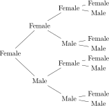
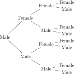
The sample space is obtained by considering all branches of this tree diagram and results in:
\(\seteqnumber{0}{4.}{0}\)\begin{align*} \Omega =&\big \{(FFFF),\,(FFFM),\,(FFMF),\,(FFMM),\,(FMFF),\,(FMFM),\\ & \,\,(FMMF),\,(FMMM),\, (MFFF),\,(MFFM),\,(MFMF),\,(MFMM),\\ & \,\,(MMFF),\,(MMFM),\,(MMMF),\,(MMMM)\big \}. \end{align*}
Each point of this space is equally likely, since the probabilities of female and male births are equal (Mendel’s laws of gamete segregation) and each element of \(\Omega \) has probability \((1/2)^4=1/16\).
-
4.2.3 The sample space for this example should portray the operational lifetime of the agricultural machines. Obviously this time is greater than or equal to \(0\), but it is also bounded. Although bounded, in practice (real life) there is no way to establish the value of this limit with certainty, and if we did, it would be an arbitrary upper limit (Mittelhammer 2013). Hence we consider the upper limit as \(+\infty \). Thus, the sample space for this case is
\(\seteqnumber{0}{4.}{0}\)\begin{align*} \Omega =& \left \{x|x\in \mathbb {R}, x\ge 0\right \}. \end{align*}
-
4.2.4 The probabilities of the events of interest are given below, using the classical measure of probability, considering the cardinalities of the events and of the sample space of exercise 4.2.2. The cardinality of \(\Omega \) is \(|\Omega |=16\) and the cardinality of an event \(A\) is represented by \(|A|\), meaning the number of elements of the subset of \(\Omega \) determined by event \(A\).
-
a) birth of at most three females:
The event of interest “birth of at most three females” is given by the subset of \(\Omega \):
\(\seteqnumber{0}{4.}{0}\)\begin{align*} A=&\big \{(FFFM),\,(FFMF),\,(FFMM),\,(FMFF),\,(FMFM),\,(FMMF),\\ & \,\,(FMMM),\,(MFFF),\,(MFFM),\,(MFMF),\,(MFMM),\,(MMFF),\\ & \,\,(MMFM),\,(MMMF),\,(MMMM)\big \}. \end{align*} Thus,
\(\seteqnumber{0}{4.}{0}\)\begin{align*} P(\textrm {birth of at most three females:}) =& P(A) = \dfrac {|A|}{|\Omega |} = \dfrac {15}{16}. \end{align*}
-
b) birth of at least three females is represented by the subset:
\(\seteqnumber{0}{4.}{0}\)\begin{align*} B=&\big \{(FFFF),\,(FFFM),\,(FFMF),\,(FMFF),\,(MFFF)\big \}. \end{align*} Thus,
\(\seteqnumber{0}{4.}{0}\)\begin{align*} P(\textrm {birth of at least three females}) =& P(B) =\dfrac {|B|}{|\Omega |}=\dfrac {5}{16}. \end{align*}
-
c) birth of exactly three females is represented by the subset \(C\) of \(\Omega \):
\(\seteqnumber{0}{4.}{0}\)\begin{align*} C=&\big \{(FFFM),\,(FFMF),\,(FMFF),\,(MFFF)\big \}. \end{align*} Therefore,
\(\seteqnumber{0}{4.}{0}\)\begin{align*} P(\textrm {birth of exactly three females}) =&P(C)=\dfrac {|C|}{|\Omega |}= \dfrac {4}{16}=\dfrac {1}{4}. \end{align*}
-
d) complementary event of \(C\), \(C^c\):
\(\seteqnumber{0}{4.}{0}\)\begin{align*} P(C^c) =&P(\textrm {birth of a number of females different from three})=1-P(C) \\ =& 1-\dfrac {1}{4}=\dfrac {3}{4}. \end{align*}
-
-
4.2.5 Example of the sampling of plant families:
-
a) The sample space is:
\(\seteqnumber{0}{4.}{0}\)\begin{align*} \Omega = & \left \{ \begin{array}{ccccc} (A,B),& (A,C),& (A,D),& (A,E),& (B,C), \\ (B,D),& (B,E),& (C,D),& (C,E),& (D,E) \\ \end {array} \right \} \end{align*}
-
b) The event \(E_1\) is:
\(\seteqnumber{0}{4.}{0}\)\begin{align*} E_1 =& \left \{(D,E)\right \}. \end{align*}
-
c) The event \(E_2\) is:
\(\seteqnumber{0}{4.}{0}\)\begin{align*} E_2 =& \left \{(A,B), (A,C), (B,C)\right \}. \end{align*}
-
d) Events \(E_1\) and \(E_2\) are mutually exclusive, since \(E_1\cap E_2\) \(=\) \(\phi \), that is, they have no outcome in common.
-
e) They are not complementary, since although they are mutually exclusive, their union does not form the sample space \(\Omega \), that is, \(E_1\cup E_2\) \(\ne \) \(\Omega \).
-
f) The event \(E_3\) is:
\(\seteqnumber{0}{4.}{0}\)\begin{align*} E_3 =& \left \{(A,B), (A,C), (A,D), (A,E) \right \}. \end{align*} The event \(E_4\) is
\(\seteqnumber{0}{4.}{0}\)\begin{align*} E_4 =& \left \{(A,D),(B,D), (C,D), (D,E) \right \}. \end{align*} i) Events \(E_3\) and \(E_4\) are not exclusive, since they have one outcome in common;
ii) \(E_3\cap E_4\) \(=\) \(\left \{(A,D)\right \}\) \(\ne \) \(\phi \), corroborating the previous statement.
-
-
4.2.6 For the example of the sampling of plant families and the events presented in the previous exercise, let us consider the classical definition of probability with a sample space with equally likely elements.
-
a) The probabilities of each event are:
\(\seteqnumber{0}{4.}{0}\)\begin{align*} P(E_1) =& \dfrac {|E_1|}{|\Omega |}= \dfrac {1}{10}=0.10,\\ P(E_2) =& \dfrac {|E_2|}{|\Omega |}= \dfrac {3}{10}=0.30,\\ P(E_3) =& \dfrac {|E_3|}{|\Omega |}= \dfrac {4}{10}=0.40,\\ P(E_4) =& \dfrac {|E_4|}{|\Omega |}= \dfrac {4}{10}=0.40.\\ \end{align*}
-
b) We have \(P(E_3\cap E_4)=\)0.10, \(P(E_4|E_3)=P(E_3\cap E_4)/P(E_3)\) \(=\) 0.10/0.40 \(=\) 0.25 and \(P(E_3|E_4)=P(E_3\cap E_4)/P(E_4)\) \(=\) 0.10/0.40 \(=\) 0.25. Thus, \(P(E_3)P(E_4|E_3)\) \(=\) 0.40\(\times \) 0.25 \(=\) 0.10 and \(P(E_4)P(E_3|E_4)\) \(=\) 0.40\(\times \) 0.25 \(=\) 0.10. Therefore, we can confirm that:
\(\seteqnumber{0}{4.}{0}\)\begin{align*} P(E_3\cap E_4) =& P(E_3)P(E_4|E_3)=P(E_4)P(E_3|E_4)=0.10, \end{align*} as expected by the properties of conditional probabilities.
-
c) The properties of probabilities are presented below. From the previous exercise we have: \(P(E_3^c)\) \(=\) \(1-P(E_3)\) \(=\) 0.60, \(P(E_4^c)\) \(=\) 0.60, \(E_3^c\) \(=\) \(\{(B,C), (B,D), (B,E), (C,D), (C,E), (D,E)\}\), \(E_4^c\) \(=\) \(\{(A,B), (A,C), (A,E), (B,C), (B,E), (C,E)\}\), \(E_3^c\cup E_4^c\) \(=\) \(\{(A,B), (A,C), (A,E), (B,C), (B,D), (B,E), (C,D), (C,E), (D,E)\}\), \(P(E_3^c\cup E_4^c)\) \(=\) \(9/10\) \(=\) 0.90. Likewise
\(\seteqnumber{0}{4.}{0}\)\begin{align*} E_3\cup E_4 =& \{(A,B),(AC),(AD),(AE),(BD),(CD),(DE)\}\\ (E_3\cup E_4)^c =& \{(BC),(BE),(CE)\}\\ (E_3\cap E_4)^c =& \{(A,B),(AC),(AE),(BD),(BC),(BE),(CE), (CD),(DE)\}\\ (E_3^c\cap E_4^c)=&\{(B,C),\,(B,E),\,(C,E)\}\\ (E_3^c\cap E_4)=&\{(B,D),\,(C,D),\,(D,E)\} \end{align*} Thus, if we use the classical definition in each case, we have the numerical verification below. In this Book we have not made algebraic (analytical) proofs of these cases.
-
i) \(P[(E_3 \cap E_4)^c]=P(E_3^c \cup E_4^c)=1-P(E_3 \cap E_4)\)
\(\seteqnumber{0}{4.}{0}\)\begin{align*} 1-P(E_3 \cap E_4)=& 0.90=1-0.10\\ 1-0.10=&0.90=0.90, \quad \textrm {Q.E.D.} \end{align*}
-
ii) \(P[(E_3 \cup E_4)^c]=P(E_3^c \cap E_4^c)=1-P(E_3\cup E_4)\)
\(\seteqnumber{0}{4.}{0}\)\begin{align*} 0.30=& 0.30= 1-0.7=0.3, \quad \textrm {Q.E.D.} \end{align*}
-
iii) \(P(E_3 \cap \phi )=P(\phi )=0\)
-
iv) \(P(E_3\cap \Omega )=P(E_3)=\)0.40
-
v) \(P(E_3\cup \phi )=P(E_3)=\)0.4
-
vi) \(P(E_3\cup \Omega )=P(\Omega )=1\)
-
vii) \(P(E_3\cap E_3^c)= P(\phi )=0\)
-
viii) \(P(E_3\cup E_3^c)= P(\Omega )=1\)
-
ix) \(P(\phi ^c)=P(\Omega )=1\)
-
x) \(P(\Omega ^c)=P(\phi )=0\)
-
xi) \(P(E_3^c)=1-P(E_3)\)
\(\seteqnumber{0}{4.}{0}\)\begin{align*} 0.60 =& 1-0.40=0.60, \quad \textrm {Q.E.D.} \end{align*}
-
xii) \(P(E_4^c)=1-P(E_4)\)
\(\seteqnumber{0}{4.}{0}\)\begin{align*} 0.40=& 1-0.60=0.40, \quad \textrm {Q.E.D.} \end{align*}
-
xiii) \(P(E_3^c\cap E_4)=P(E_4)-P(E_3\cap E_4)\)
\(\seteqnumber{0}{4.}{0}\)\begin{align*} 0.30 =& 0.40 - 0.10=0.30, \quad \textrm {Q.E.D.} \end{align*}
-
-
d) Since \(P(E_3|E_4)=\)0.25 \(\ne \) \(P(E_3)\) and, likewise, \(P(E_3\cap E_4)=\)0.1 \(\ne \) \(P(E_3)P(E_4)=\)0.16, then events \(E_3\) and \(E_4\) are not independent.
-
e) Since \(E_1\) and \(E_3\) are exclusive, they are not independent. This is a common confusion among many readers: not distinguishing between mutually exclusive and independence. In fact, if two events are exclusive, they cannot be independent. Otherwise, since \(P(E_1\cap E_3)=\)0.00 \(\ne \) \(P(E_1)P(E_3)\) \(=\) 0.04, events \(E_1\) and \(E_3\) are not independent.
-
-
4.2.7 Example of the marker gene \(B\) and resistance gene \(A\):
-
a) To be resistant the event regarding the genotypes must be \(AA\) or \(Aa\), since the dominant allele \(A\) confers resistance and allele \(a\) is recessive. We call these genotypes simply \(A-\). The previous Table relates this event to the genotypes by calling it the “Resistant” phenotype. The susceptible phenotype refers to the \(aa\) phenotype. This table is a summary of a more complex table (shown in the last exercise) of the joint distribution of the two genes regarding their possible genotypic classes. If we denote the event “being resistant” by \(R\) and the marker genotype \(BB\) as the other event. Thus, we want \(P(R|BB)\), which depends on the event \(R\cap BB\). The probability of this case is \(P(R\cap BB)\) \(=\) \((1-r^2)/4\). Thus,
\(\seteqnumber{0}{4.}{0}\)\begin{align*} P(R|BB) =& \dfrac {P(R\cap BB)}{P(BB)}=\dfrac {(1-r^2)/4}{(1-r^2)/4+ r^2/4}=1-r^2. \end{align*}
-
b) The desired graph:
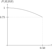
If the genes are independent \((r=0.5)\), this probability is 0.75. This is the expected frequency in an \(F_2\) generation, for the genotypes \(AA\) (0.25) and \(Aa\) (0.50), looking marginally at the segregation of gene \(A\). Thus, the marginal probability is equal to the conditional probability. If \(r<\)0.5, the probability \(P(R|BB)>\)0.75, increasing the chance of selecting genotypes related to resistance.
-
c) The complete table of the genotypic distribution is given below with the probabilities given in each cell:
Marker genotype B Genotype(A) \(BB\) \(Bb\) \(bb\) \(AA\) \((1-r)^2/4\) \(r(1-r)/2\) \(r^2/4\) \(Aa\) \(r(1-r)/2\) \((1-r)^2/2\) \(+\) \(r^2/2\) \(r(1-r)/2\) \(aa\) \(r^2/4\) \(r(1-r)/2\) \((1-r)^2/4\)
The required probability is: \(P(AA|BB)\) \(=\) \(P(AABB)/P(BB)\) \(=\) \((1-r)^2/4/(1/4)\) \(=\) \((1-r)^2\), since \(P(BB)\) \(=\) \((1-r)^2/4\) \(+\) \(r(-r)/2\) \(+\) \(r^2/4\) \(=\) \(1/4\). If we redo the graph for this case, we have:
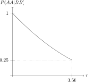
If the genes are independent \((r=\)0.5\()\), this probability is 0.25. This is the expected frequency in an \(F_2\) generation, for the genotypes \(AA\) (0.25), looking marginally at the segregation of gene \(A\). Thus, the marginal probability is equal to the conditional probability. If \(r<\)0.5, the probability \(P(AA|BB)>\)0.25, increasing the chance of selecting genotypes related to resistance in the genotypic class \(AA\) only. This procedure is often used, since in real life we cannot see the genotypes of the plants regarding the genes of interest (the resistance gene in this case) and often we cannot even select by phenotype, due to the impossibility of inoculating the microorganism in the field. Therefore, we take a linked marker and select through it. The greater the linkage, that is, the closer to \(0\) \(r\) is, the greater the chance of being successful in obtaining a favorable genotype among those selected by the marker genotype (which we can see using laboratory techniques).
-